
The decision tree is one of the most commonly used algorithms in supervised learning. You can use it for both regression and classification when we use this algorithm for regression problems, it is called a regression tree.
In real life, decision trees are very famous algorithms they are used to predict high occupancy dates for hotels, see gross margins of companies, select which flight to travel on, and the list goes on and on.
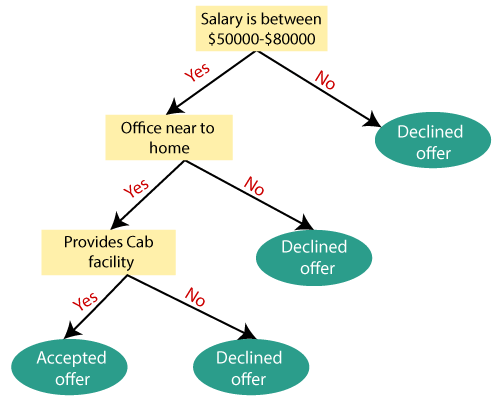
Now, what is a decision tree? Thinking intuitively, we might conjure up an image like this.
In certain situations of life, we think in decision trees,
For example: Handling a midnight craving for food.
This is a perfect intuition for a decision tree.
A decision tree is a collection of nodes and branching that is a hierarchical structure that tries to come to a conclusion by using a variety of questions at different stages.
To understand the regression tree, we need to understand a few terms before:-
- Node – in the figure above, the yellow circles denote a node. The nodes play an integral part in decision-making. It’s the node where the algorithm decides which pathway to choose further.
- Root node – The root node is the starting node or the topmost node from where the tree originates. It acts as a starting point for the algorithm.
- Leaf node – The final node or the output node, which acts as the termination point in the algorithm, is known as the leaf node.
If the decision tree asks logical questions at each node, how can it predict the continuous values?
We know regression algorithms use RSS (residual sum of squares, i.e. )to predict the accuracy, so what the regression tree will do will ask at each node whether this step reduces the RSS or not
Let’s consider an example let the data be
| X | Y |
| 1 | 1 |
| 2 | 1.2 |
| 3 | 1.3 |
| 4 | 1.5 |
| 5 | 1.5 |
| 6 | 5 |
| 7 | 5.7 |
| 8 | 5.6 |
| 9 | 5.4 |
| 10 | 5.9 |
| 11 | 15 |
| 12 | 15.4 |
| 13 | 15.2 |
| 14 | 15.8 |
| 15 | 15.6 |
| 16 | 7.7 |
| 17 | 7.5 |
| 18 | 7.11 |
| 19 | 7.4 |
| 20 | 7.9 |
If we try to plot this data
Notebook to run and test code: https://www.kaggle.com/code/tanavbajaj/decision-tree/notebook
| import numpy as np import matplotlib.pyplot as pltx = np.array(range(1,21)) y = np.array([1,1.2,1.3,1.5,1.2,5,5.7,5.6,5.4,5.9,15,15.4,15.2,15.8,15.6,7.7,7.5,7.11,7.4,7.9])plt.scatter(x,y) plt.show |
Now let us try to apply linear regression to this
| from sklearn.linear_model import LinearRegression x = x.reshape(-1,1)Y = y.reshape(-1,1)reg = LinearRegression().fit(x, y) y_pred = reg.predict(x)plt.scatter(x, y) plt.plot(x, y_pred, ‘r’) plt.title(‘Best fit line using linear regression model from sklearn’) plt.xlabel(‘x-axis’) plt.ylabel(‘y-axis’)plt.show() |
We can observe that the best line does not capture all the points well; in this scenario, a decision tree would be a better option.
How does the regression tree work?
It starts by taking the average of the first 2 values and splits the data based on the average of the data points after this; it will try and predict all the values based on this split line and calculate RSS error for this line. It will then take the average of the second and third and recalculate the RSS. it will repeat this process for all the data points and then select the line for the value which would give the least RSS.
Ultimately, our tree will end up splitting nodes for all the values in the tree. Is this a good thing? No, if we visualize this.
It will look something like this which is far from the best plot which might look something like
As the first graph is far too overfitted and might lead to wrong results, how can we avoid overfitting?
We can stop the overfitting by specifying the depth of the tree, which is the minimum number of elements to have before the slit is conducted in other words, when the tree is created, what should be its height between the root node and leaf node.
Now let’s see how a regression tree performs better than linear regression in some case
If we try to retrain data using linear regression and plot the test output against test predictions, we get a plot like
| from sklearn.model_selection import train_test_split X_train, X_test, y_train, y_test = train_test_split( x, y, test_size=0.25,random_state=55)from sklearn.linear_model import LinearRegressionreg = LinearRegression().fit(X_train,y_train) y_pred_lr = reg.predict(X_test)plt.scatter(X_test,y_test,color=”red”) plt.scatter(X_test,y_pred_lr,color = “blue”) plt.show() |
The blue dots are the test dataset, and the red is linear regression predictions.
In the same graph, if we import the decision tree from sklearn and plot it against the test data, we might get a plot like
| from sklearn.tree import DecisionTreeRegressor
regressor = DecisionTreeRegressor(random_state=4,max_depth=3) |
We can see the predicted results are closer to the actual value
In this graph, red dots denote the actual value, green dots denote the value predicted by the regression tree, and blue dots the value predicted by linear regression
Now let’s visualize the decision tree built by the algorithm
| from sklearn.tree import export_graphviz export_graphviz(regressor, out_file =’tree.dot’, feature_names =[‘x value’]) |
We get this decision tree which is used by the algorithm.
This image shows what the algorithm thinks at every node.
A combination of decision trees gives us a random forest algorithm, which is the topic for the next release.
Pruning and Regularization: Understanding the Techniques for Pruning and Regularizing Decision Trees
Understanding the Techniques for Pruning and Regularizing Decision Trees
Decision trees have the tendency to grow to their full depth, which can result in overfitting. Pruning and regularization techniques are employed to prevent overfitting and improve the generalization capabilities of decision trees.
Pruning involves the removal of specific branches or nodes from a decision tree to simplify its structure and reduce complexity. The goal of pruning is to find the optimal tradeoff between model simplicity and predictive performance. One common pruning technique is post-pruning, where the tree is initially grown to its maximum depth and then pruned back based on certain criteria, such as the reduction in impurity or the increase in accuracy.
Regularization, on the other hand, aims to add constraints or penalties to the learning process to prevent overfitting. Regularization techniques introduce additional parameters or modify the splitting criteria to control the tree’s growth. One popular regularization technique is cost complexity pruning or minimal cost-complexity pruning, which uses a complexity parameter to control the size of the tree during the learning process.
Both pruning and regularization techniques help prevent overfitting by limiting the complexity of decision trees. By reducing unnecessary branches or nodes, these techniques improve the generalization capabilities of the model and allow it to perform better on unseen data. However, it is important to find the right balance between complexity reduction and model accuracy to ensure optimal results.
Dealing with Missing Values: Strategies for Handling Missing Values in Decision Trees
Handling missing values is an essential step in building decision trees, as missing data can significantly impact the accuracy and reliability of the model. Fortunately, decision trees offer several strategies to deal with missing values effectively.
One common approach is to perform surrogate splitting, where surrogate splits are created to handle missing values. Surrogate splits consider alternative splitting rules for missing data based on the correlations between predictor variables. These surrogate splits allow decision trees to still make predictions for instances with missing values by considering the relationships with other variables.
Another strategy is to treat missing values as a separate category or create a separate branch for instances with missing data. This approach ensures that missing values are explicitly accounted for during the decision-making process, allowing the model to make informed predictions for such instances.
Additionally, decision trees can employ imputation techniques to estimate missing values. Imputation involves filling in missing values based on statistical measures such as mean, median, or mode. By imputing missing values, decision trees can utilize the complete dataset and avoid the exclusion of valuable information.
It is important to consider the nature of the missing data and the characteristics of the dataset when selecting the appropriate strategy for handling missing values in decision trees. Careful preprocessing and imputation methods can help maintain the integrity of the data and enhance the performance of the model.
Interpretability and Explainability: Examining the Interpretability and Explainability of Decision Trees
One of the key advantages of decision trees is their interpretability and explainability. Decision trees provide a clear and intuitive representation of the decision-making process, making them highly interpretable.
The structure of a decision tree can be easily understood and visualized, with each node representing a decision based on a specific feature or attribute. The path from the root node to a leaf node represents the series of decisions leading to a final prediction. This transparency allows domain experts and stakeholders to grasp the underlying reasoning behind the model’s predictions.
Decision trees also offer feature importance measures, such as Gini importance or information gain, which quantify the contribution of each feature to the decision-making process. These measures provide insights into the relative importance of different variables, aiding in feature selection and understanding the relationships between features and outcomes.
Furthermore, decision trees can generate easily interpretable rules that describe decision boundaries and classification criteria.
Overfitting and Underfitting: Analyzing the Tradeoff between Overfitting and Underfitting in Decision Trees
Decision trees, like any other machine learning models, are susceptible to overfitting and underfitting. Overfitting occurs when a decision tree captures noise or irrelevant patterns in the training data, resulting in poor generalization to new, unseen data. On the other hand, underfitting happens when a decision tree fails to capture the underlying patterns in the data, leading to high bias and low predictive performance.
Overfitting can be a consequence of decision trees’ ability to create complex and detailed decision boundaries. When a decision tree grows too deep, it becomes highly sensitive to small fluctuations in the training data, capturing noise and outliers. This results in a model that performs well on the training set but fails to generalize to new data.
To combat overfitting, various techniques can be employed. One common approach is to limit the depth of the decision tree, also known as tree pruning, by imposing constraints on the tree’s growth. Another technique is to set a minimum number of samples required to split a node or to merge nodes, which helps prevent the tree from creating small, spurious branches.
Underfitting, on the other hand, occurs when the decision tree is too simplistic and fails to capture the complexities of the underlying data. This can happen when the tree is not allowed to grow deep enough or when the splitting criteria are not effective in capturing the relationships between features and the target variable.
Finding the right balance between overfitting and underfitting is crucial for optimal model performance. Regularization techniques, such as adjusting hyperparameters like the maximum tree depth, minimum sample split, or minimum impurity decrease, can help strike this balance. Additionally, you can use cross-validation techniques to evaluate the model’s performance on unseen data. Moreover, you can guide the selection of appropriate hyperparameters.
Ensemble Methods: Exploring Ensemble Methods that Utilize Decision Trees, such as Random Forest and Gradient Boosting
Ensemble methods combine multiple decision trees to improve prediction accuracy and reduce the risk of overfitting. Two popular ensemble methods that utilize decision trees are Random Forest and Gradient Boosting.
Random Forest is an ensemble technique that constructs a collection of decision trees and aggregates their predictions through voting or averaging. In a Random Forest, each decision tree is trained on a distinct subset of the training data and considers only a random subset of features for each split. This randomness helps to decorrelate the individual trees and reduce overfitting, resulting in improved generalization performance.
Gradient Boosting, on the other hand, builds decision trees sequentially, where each subsequent tree corrects the mistakes made by the previous tree. Gradient Boosting optimizes a loss function by iteratively adding decision trees, each focusing on the residuals or errors of the previous trees. By combining weak learners (shallow trees) in a boosting framework, Gradient Boosting can create a strong learner with high predictive power.
Both Random Forest and Gradient Boosting have proven to be powerful and effective methods for various machine learning tasks. They are robust against overfitting, handle high-dimensional data well, and are capable of capturing complex relationships between features and the target variable.
Practical Applications: Examining Real-World Use Cases and Applications of Decision Trees
Decision trees have found widespread application across various industries due to their simplicity, interpretability, and ability to handle both categorical and numerical data. Here are some real-world use cases where you can see successfully employ decision trees:
Customer Relationship Management (CRM):
In CRM systems, decision trees often segment customers based on attributes like demographics, purchasing behavior, and preferences. These segments can then help personalize marketing campaigns, optimize product recommendations, and enhance customer satisfaction.
Credit Risk Assessment:
You can utilize decision trees in the banking and financial sector for credit risk assessment. By analyzing factors such as credit history, income, employment status, and debt levels, decision trees can accurately predict the likelihood of loan default or creditworthiness of applicants.
Fraud Detection:
Decision trees play a crucial role in detecting fraudulent activities across industries, including banking, insurance, and e-commerce. By analyzing patterns and variables associated with fraudulent behavior, decision trees can help identify suspicious transactions, fraudulent claims, or fraudulent user activities.
Manufacturing and Quality Control:
You can employ the decision trees in manufacturing processes to ensure quality control and identify potential defects. By analyzing input variables such as temperature, pressure, and machine settings, decision trees can classify products as defective or non-defective, aiding in reducing waste and optimizing production efficiency.
Medical Diagnosis:
You can use decision trees in medical diagnosis systems to assist doctors in identifying diseases or conditions depending upon patient symptoms, medical history, and test results. Decision trees provide a structured approach to decision-making, helping medical professionals make accurate diagnoses and determine appropriate treatment plans.
Conclusion
Decision trees are versatile and powerful machine learning models with a wide range of applications across industries. Their simplicity, interpretability, and ability to handle various data types make them valuable tools for solving complex problems.
Practitioners can effectively leverage decision trees in their specific use cases by understanding the tradeoff between overfitting and underfitting, employing ensemble methods such as Random Forest and Gradient Boosting, addressing missing values, and considering the interpretability and explainability of decision trees.
However, it is important to note that decision trees may not always be the best choice for every scenario. They have limitations, such as their tendency to create complex decision boundaries and their sensitivity to small fluctuations in data. It is essential to carefully evaluate the characteristics of the problem at hand, the available data. The desired objectives before deciding to use decision trees or exploring alternative machine learning approaches.
Overall, decision trees are valuable tools. It continues to find practical applications in diverse industries, offering insights, predictions, and actionable information for decision-making. With their intuitive nature and ability to handle both structured and unstructured data, decision trees remain an essential component of the machine learning toolkit.
FAQs
What is a Decision Tree in regression?
A Decision Tree in regression is a machine learning algorithm used for predictive modeling.
How does a Decision Tree regression work?
It partitions the feature space into regions and predicts the target variable based on the average value of observations within each region.
When should I use Decision Tree regression?
Use Decision Tree regression for predicting continuous outcomes with nonlinear relationships.
How does Decision Tree regression handle overfitting?
It can overfit the training data, but techniques like pruning or setting maximum depth help mitigate overfitting.
Can Decision Tree regression handle missing data?
Yes, it can handle missing data by splitting nodes based on available features.
How do I interpret the results from a Decision Tree regression model?
Interpret the model by examining how features are used to partition the data and their impact on predicting the target variable.
Is Decision Tree regression suitable for large datasets?
Decision Tree regression can handle large datasets efficiently due to its ability to partition data iteratively.