
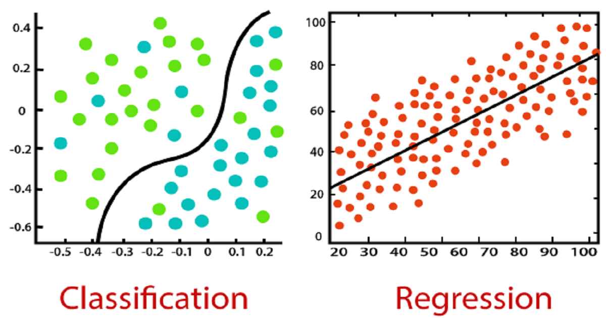
Under supervised learning, there is a type called classification. These algorithms recognize the category a new observation belongs to based on the training dataset. In supervised learning, there are independent variables and a dependent variable Here, the dependent variable is the category, and each category’s features are independent variables. These categories are distinct and pre-defined such as True or False, is the email is “spam” or “not,” does the picture have “trees” or “not,” etc.
The above diagram is a case of successful classification where the circles and triangles are in separate classes based on their features.
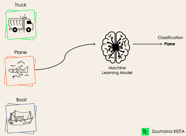
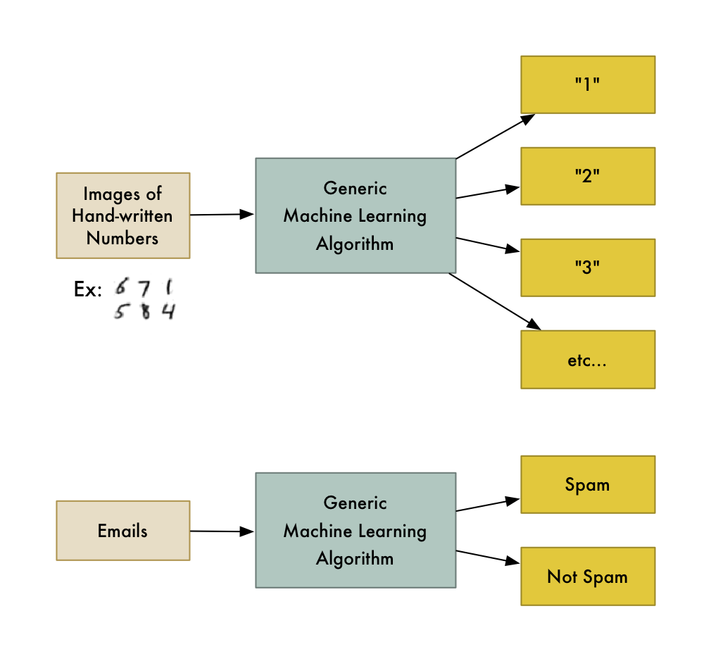
The most common classification problems are speech recognition, handwriting recognition, and face detection. These can be a binary classification or multi-class classification problems.
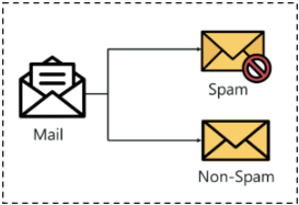
Examples of classification:
Classification of Email into “spam” and “not spam.”
Classification is a 2 step process.
First is training the model and then testing its accuracy. First, a classifier is built based on the training dataset. The classifier analyses the dataset and associated labels. After analyzing it creates some prediction rules.
Secondly, these rules are tested upon unseen data, also called testing data. Then the accuracy of the classifier is calculated; if the accuracy is not good on the test data, the ML model will reframe until it gets optimized.
The accuracy is determined by checking the percentage of the dataset correctly classified by the classifier.
Note: Before blindly applying a classifier to the dataset, check the ratio of each category in the training dataset; if any category is less, the training rules might have issues. In an ideal case, the dataset contains an equal amount of data for each category.
Let’s take an example with code to understand this better.
SONAR Dataset: Rocks Vs. Mine Classification
To run and check the code:
SONAR is a device that uses sound waves to detect objects in the ocean. Depending on different types of frequencies, the object is detected.
The dataset here contains 60 frequencies detected by the SONAR and one column containing information on whether the object is a rock or a mine.
This information is crucial for most ships in the war because if a rock is present at that location, it is safe to pass over it, and if a mine is present, that is potentially dangerous.
The first step for every python project is importing the modules required.
Importing Python Modules:
Here Numpy and Pandas are used to read the data and help in preprocessing.
Sklearn is the library that contains modules for train_test_spilt, LogisticRegression, and accuracy_score.
Train_test_split, as the name shows, is used to split the dataset into training and testing data.
Logistic Regression is the classification algorithm being used in this example. (More detail on this in further articles.)
Reading Data:
| sonar_data = pd.read_csv(‘../input/connectionist-bench-sonar-mines-vs-rocks/sonar.all-data.csv’, header=None) |
Pandas is used to read the data from the CSV file.
| sonar_data[60].value_counts() |
As mentioned above, it is important to check whether the data for each category is enough.
Output:
It shows that 111 out of 208 tuples are in the mining category, and 97 are for rock.
So, 46% of the data is for rocks and 54% for mines which is sufficient for moving forward.
Some preprocessing is done where some unnecessary columns and rows are dropped.
| X = sonar_data.drop(columns=60, axis=1) Y = sonar_data[60] X=X.drop([0]) Y=Y.drop([0]) |
Train Test Split:
| X_train, X_test, Y_train, Y_test = train_test_split(X, Y, test_size = 0.25, random_state=1) |
As seen in the code the dataset is split into training and testing datasets.
The test_size=0.25 shows that 75% of the dataset will be used for training while 25% for testing.
Training the model:
| model = LogisticRegression() model.fit(X_train, Y_train) |
Sklearn makes it very easy to train the model. Only 1 line of code is required to do so.
Checking Accuracy:
| X_train_prediction = model.predict(X_train) training_data_accuracy = accuracy_score(X_train_prediction, Y_train) |
This code is used to check the accuracy of the training dataset.
| X_test_prediction = model.predict(X_test) test_data_accuracy = accuracy_score(X_test_prediction, Y_test) |
This code is used to test out the accuracy of the testing dataset.
An accuracy of 83% for training and 80% for testing datasets is pretty good for a basic classification algorithm.
Now let’s add some random data and check what the model predicts.
| input_data = (0.0307,0.0523,0.0653,0.0521,0.0611,0.0577,0.0665,0.0664,0.1460,0.2792,0.3877,0.4992,0.4981,0.4972,0.5607,0.7339,0.8230,0.9173,0.9975,0.9911,0.8240,0.6498,0.5980,0.4862,0.3150,0.1543,0.0989,0.0284,0.1008,0.2636,0.2694,0.2930,0.2925,0.3998,0.3660,0.3172,0.4609,0.4374,0.1820,0.3376,0.6202,0.4448,0.1863,0.1420,0.0589,0.0576,0.0672,0.0269,0.0245,0.0190,0.0063,0.0321,0.0189,0.0137,0.0277,0.0152,0.0052,0.0121,0.0124,0.0055)
# changing the input_data to a numpy array # reshape the np array as we are predicting for one instance prediction = model.predict(input_data_reshaped) |
Here some random input data was added and then reshaped using numpy to be used as input for the model.
The model predicts that this input dataset means that the ship is near a mine and should not move on top of it.
In summary, the logistic regression model, when trained on the training dataset and tested on the testing dataset, demonstrated an accuracy of 84% for training data and 80% for testing data. This indicates that the model is capable of accurately predicting whether an object is a mine or a rock based on random input data.
In the vast field of machine learning and data analysis, classification is a fundamental concept that plays a crucial role in various applications. Classification involves the process of categorizing or classifying data into distinct groups or classes based on specific characteristics or features. It is a supervised learning task where the goal is to predict the class or category of a given input based on a set of labeled examples.
The need for classification arises in numerous domains, including image recognition, spam filtering, sentiment analysis, medical diagnosis, fraud detection, and more. By employing classification algorithms, we can automatically classify new, unseen data into predefined classes, making it an essential tool for decision-making and pattern recognition.
The Basics of Classification
At its core, classification involves two key components: the features and the labels. Features are the measurable characteristics or attributes of the data that help distinguish one class from another. For instance, in email spam detection, features may include the presence of certain keywords, the sender’s address, or the email’s content. Labels, on the other hand, represent the predefined classes or categories that we want to assign to the data, such as “spam” or “not spam.”
To create a classification model, we typically start with a labeled dataset called the training set. The training set consists of a collection of data instances, each associated with its corresponding label. The classification algorithm learns patterns and relationships within the training data, enabling it to make predictions on unseen instances. Once you train the model, you can use it to classify new, unlabeled data based on the learned patterns.
Types of Classification Algorithms:
There is a wide range of classification algorithms available, each with its own strengths, weaknesses, and areas of application. Some popular classification algorithms include:
- Decision Trees: Decision trees create a hierarchical structure of decisions based on the features. Each internal node represents a decision based on a particular feature, while the leaf nodes correspond to the class labels. Decision trees are easy to interpret and can handle both categorical and numerical features.
- Random Forest: Random Forest is an ensemble learning method that combines multiple decision trees. It creates a diverse set of decision trees and combines their predictions to make the final classification. Random Forest often exhibits high accuracy and can handle large datasets.
- Support Vector Machines (SVM): SVM is a powerful algorithm for binary classification. It separates data instances by finding the optimal hyperplane that maximizes the margin between different classes. SVMs can handle complex datasets and are effective even in high-dimensional spaces.
- Naive Bayes: Naive Bayes is a probabilistic algorithm based on Bayes’ theorem. It assumes that features are conditionally independent given the class labels, hence the “naive” assumption. Naive Bayes is computationally efficient, particularly with large datasets, and performs well in text classification and spam filtering tasks.
- Logistic Regression: Despite its name, logistic regression is a classification algorithm that you can use for binary and multiclass problems. It models the relationship between the features and the probability of belonging to a particular class using a logistic function. Logistic regression is simple, interpretable, and widely used in various applications.
Evaluation and Performance Metrics:
Evaluating the performance of a classification model is crucial to assess its effectiveness and generalization capability. Common evaluation metrics include accuracy, precision, recall, and F1-score.
- Accuracy measures the overall correctness of the model’s predictions, i.e., the ratio of correctly classified instances to the total number of instances.
- Precision measures the proportion of correctly predicted positive instances among all instances predicted as positive. It focuses on the correctness of positive predictions.
- Recall (also known as sensitivity or true positive rate) measures the proportion of correctly predicted positive instances among all actual positive instances. It focuses on capturing all positive instances.
- F1-score combines precision and recall into a single metric by taking their harmonic mean. It provides a balanced measure of a model’s performance.
Conclusion
Choosing the appropriate evaluation metric depends on the nature of the problem and the relative importance of different types of errors. For instance, in medical diagnosis, recall may be more crucial to avoid false negatives, while in spam filtering, precision might be more important to minimize false positives.
Conclusion Classification is a fundamental task in machine learning and data analysis. By categorizing data into distinct classes based on specific features, classification algorithms enable us to make predictions and decisions in various domains. With a wide range of classification algorithms available and various evaluation metrics to assess their performance, classification continues to be a critical tool for extracting insights and patterns from data.
FAQs
What is classification?
Classification is the process of organizing data into categories or groups based on certain characteristics or features.
Why is classification important?
Classification helps in organizing and understanding large amounts of data, making it easier to analyze and derive insights from.
What are the common techniques used in classification?
Common techniques include decision trees, support vector machines, logistic regression, k-nearest neighbors, and neural networks.
How does classification differ from clustering?
Classification assigns predefined labels to data, while clustering groups similar data points together without predefined labels.
What are some real-world applications of classification?
Classification is used in spam email detection, sentiment analysis, medical diagnosis, fraud detection, and image recognition.
What is the process of building a classification model?
The process involves selecting and preprocessing data, choosing a suitable algorithm, training the model on labeled data, and evaluating its performance.
How do you measure the performance of a classification model?
Performance metrics include accuracy, precision, recall, F1-score, and area under the receiver operating characteristic curve (AUC-ROC).