
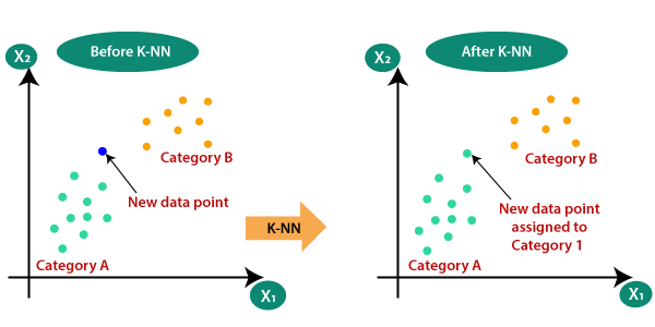
K Nearest neighbour (KNN) is one of the most basic classification algorithms. It follows the assumption that similar things exist in close proximity to each other.
The K-nearest neighbour algorithm calculates the distance between the various points whose category is known and then selects the shortest distance for the new data point. It is an algorithm that comes under supervised learning scenarios, which means we already have the predefined classes available.
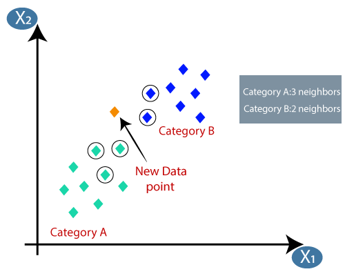
The K in the KNN algorithm refers to the number of the neighbours considered. This can take any whole number as input.
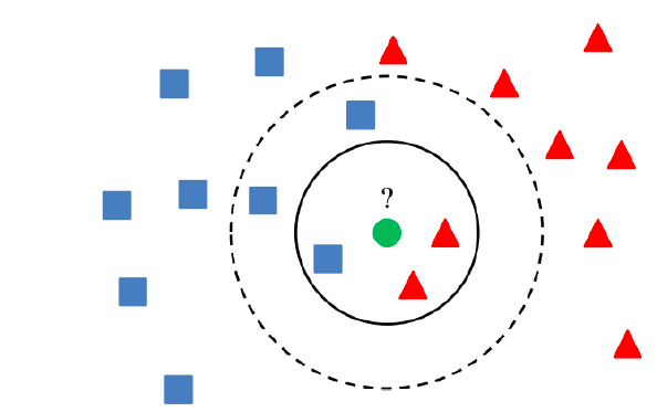
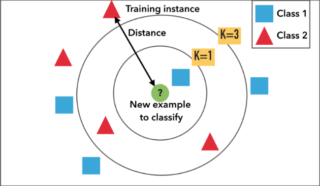
Consider an example that shows whether a certain product is normal or has an anomaly, where blue squares show the normal product, and red triangles are anomalies. Green circles are the product that we want to predict. In this case, if we consider the value of K to be 3, i.e., inner circle, the object is classified as an anomaly due to vote out by the triangle. Still, if we consider K = 5, the product is classified as normal due to most blue squares.
To conclude, we can say in simpler terms that KNN takes the nearest neighbors of the point and tries to classify it based on most of the closest points.
HOW TO CONSIDER DISTANCES BETWEEN POINTS?
Certain distances are commonly used while using the KNN algorithm.
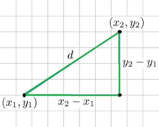
- Euclidean Distance:-
Consider 2 points and so the euclidean distance between them would be. This distance denotes the shortest distance between the two points it is also known as Norm.

2. Manhattan distance:-
Manhattan distance refers to the sum of the absolute difference between the points
3.Minkowski distance:-
For the distance between two points, it is calculated as
If we make p = 1, it becomes Manhattan distance, and when p = 2, it becomes euclidean distance.
How to select the value of K?
Before we dive into understanding how to select the optimal value of K, we need to understand what decision boundary means.
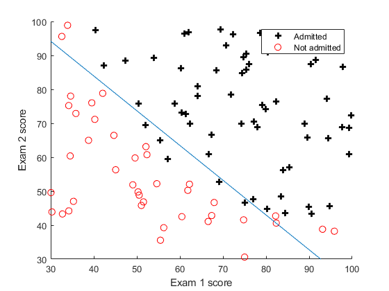
Consider a data set consisting of circles and pus labels so if we try to generalize the relation or the pattern of classification, we can draw a line or a curve as drawn by the blue line, which easily separates the majority of plus and the circles. The curve acts as a guide to the algorithm in classifying the point. The curve is known as the decision boundary.
Now, if we consider another data set that has points in the following distribution and considers
K = 1, then the decision boundary will be something like
And if the test point is closer to the center circle, it would be classified as a circle rather than a cross that is in the majority around the center. Such kind of model is known as an overfitted model
In another case, if we consider the value of K to be very large, we may end up classifying everything as square as the decision boundary would tend more towards the majority of the label, which being square; in this case, such a model is known as underfit model thus it is important to select the optimal value of K
Now we may ask how we can calculate perfect K.
To answer that, there is no step-by-step process to calculate the perfect value of the K.
To calculate the value of the K, we will have to go by approximation and guess and to find the best match.
Let’s understand this with an example.
As usual, let’s start with importing the libraries and then reading the dataset:
| from sklearn import datasets from sklearn.neighbors import KNeighborsClassifier from sklearn.model_selection import train_test_split |
| dataset = datasets.load_breast_cancer() |
This data set contains the data about whether a cancer is malignant or not.
| X_train , X_test , Y_train , Y_test = train_test_split(dataset.data , dataset.target , test_size = 0.2,random_state=0) |
We then split data into training and testing datasets
| clf = KNeighborsClassifier() clf.fit(X_train, Y_train) |
Next, we select the classifier as Kneigbor and fit it using X_train and Y_train data
| clf.score(X_test, Y_test) |
0.9385964912280702
Upon scoring the algorithm, we get a score of .93
By default, KNN selects the value of K to be 5.
Now we may argue to change the score; we can try and set the value of K to some different number and then rerun over the test data to increase the score. Still, in reality, we are trying to fit the test data into the model, which in the end, would defeat the purpose of the test data.
As an alternative, we may say that what if we try to train the algorithm using training data and then repass it as test data to decide the optimum value of K. Still, in that case, we will end up getting a 100% accuracy over training data. Still, it will fail on the test data and give low scores.
Cross-validation and
Validation

Now to find the optimum value of K, what we can do is take our training data and split it into two parts in a 60:40 ratio then we can use the 60% of the data to train our model and the remaining 40% of the training data to test and determine the value of K without compromising the integrity of the Test data. This process is known as Cross-validation.
However, it is also said that the more the training data is available, the better is the model, but we already lost 40% of our data to testing cases to overcome this, we use K fold cross-validation.
Consider we have a box denoting our training data.
Then k fold cross validation states that we can split our training data into P number of parts and use P -1 parts for training and the remaining 1 for testing purposes.
In simpler words, we can use 1 part at a time for testing and the remaining for training, i.e., if we considered 1st part for testing, then from 2nd part onwards up to the end will be used for training purposes, the next 2nd part would be considered for testing and remaining parts would be considered for training, so on and so forth.
After calculating the scores of various parts, we can take an average of the scores and consider it as the score for the particular value of K.
Let’s see this using an example.
Continuing on the above example where the breast cancer dataset was chosen.
Now to implement K fold CV, we use a for loop and repeatedly score the data for the various values of K and store them in an array so it would be easier to plot using matplotlib
| x_axis = [] y_axis = [] for i in range(1, 26, 2): clf = KNeighborsClassifier(n_neighbors = i) score = cross_val_score(clf, X_train, Y_train) x_axis.append(i) y_axis.append(score.mean()) |
We use odd values of the K while considering the values of K assume in the neighbor of the unknown point; we get an equal number of labels A or label B it would be difficult to classify. Thus, to avoid it, we consider an odd number of neighbours.
| import matplotlib.pyplot as plt plt.plot(x_axis, y_axis) plt.show() |
We import matplotlib and plot the variation of the score against the various value of K
From this plot, we come to know that the best accuracy comes near K = 7 Thus, we will consider K as 7.
Now let’s try to implement this algorithm from scratch by ourselves
Using K fold CV we came to know that we would get the best result at K = 7 so let’s run the algorithm using K = 7 and score it on the same random state using sklearn
| from sklearn import datasets from sklearn.neighbors import KNeighborsClassifier from sklearn.model_selection import train_test_split |
Importing libraries and dataset from sklearn
| dataset = datasets.load_breast_cancer() X_train, X_test, Y_train, Y_test = train_test_split(dataset.data, dataset.target, test_size = 0.2, random_state = 0) |
Loading dataset and splitting the data into training and testing data in an 80:20 ratio, since we would be trying to implement this algorithm ourselves, we are splitting data using a particular random state to get some split every time
| clf = KNeighborsClassifier(n_neighbors=7) clf.fit(X_train, Y_train) |
Calling the classifier and specifying the value of K as 7 then we call the fit function so as to train the model
| clf.score(X_test, Y_test) |
Upon scoring the algorithm, we get a score of
0.94736842105263153
Limitation of KNN
KNN’s limitations: KNN is an extremely strong algorithm. It is also known as a “slow learner.” It does, however, have the following limitations:
- Doesn’t function well with huge datasets: Because KNN is a distance-based method, the cost of computing the distance between a new point and each old point is quite high. This degrades the algorithm’s speed.
- Doesn’t function well with many dimensions: Same as above. The cost of calculating distance increases in higher dimensional space, affecting performance.
- Sensitive to outliers and missing data: Because KNN is sensitive to outliers and missing values, we must first impute missing values and remove outliers before using the KNN method.
K-Nearest Neighbors (K-NN) is a popular algorithm that you can use in machine learning for both classification and regression tasks. It is a non-parametric method that determines the classification or prediction of a new data point based on the majority vote or average of its k nearest neighbors in the feature space.
The algorithm works as follows:
- Dataset Preparation: To apply the K-NN algorithm, you must prepare the dataset. It should include labeled data points, where each data point has a set of features and a corresponding class or target variable. It is important to normalize or standardize the features to ensure that no single feature dominates the distance calculations.
- Determining the Value of k: Selecting the appropriate value for k, the number of neighbors to consider, is a crucial step. As a hyperparameter, you can determine the optimal value of k through trial and error or by employing techniques such as cross-validation, ensuring it is best suited to address the specific problem at hand. A small k value might lead to overfitting, while a large k value may lead to oversimplification.
Calculating Distances:
For a new data point, the algorithm calculates the distances between the data point and all other data points in the training set using a distance metric such as Euclidean distance, Manhattan distance, or Minkowski distance. The distance metric chosen depends on the nature of the data and the problem at hand.
Identifying the Neighbors:
The algorithm identifies the k nearest neighbors of the new data point based on calculated distances. You can select the data points with the shortest distances to the new point.
Classification or Regression
– For classification tasks, it determines the class label of the new data point based on the majority class among its k nearest neighbors, with each neighbor’s class having equal weight in the voting process.
– For regression tasks, it predicts the value of the new data point by averaging the target variable values of its k nearest neighbors.
Handling Ties:
In cases of a tie in majority voting for classification or the average value for regression, the algorithm may employ techniques like weighted voting or consider additional neighbors to break the tie and make a final prediction.
K-NN offers several advantages:
- Simplicity: The algorithm is simple to understand and implement. This makes it an accessible choice for beginners in machine learning.
- No Training Phase: K-NN is a lazy learner, meaning it does not require a training phase. The model directly uses the training data during the prediction phase. This makes it easy to update the model with new data.
- Non-parametric: K-NN does not make assumptions about the underlying data distribution. This makes it suitable for a wide range of data types and problem domains.
- Versatility: you can apply K-NN to both classification and regression tasks. This makes it a versatile algorithm that can handle different types of problems.
However, K-NN also has limitations:
- Computational Complexity: The algorithm requires calculating distances between the new data point and all other data points in the training set, which can be computationally expensive for large datasets. This makes K-NN less suitable for real-time or large-scale applications.
- Sensitivity to Feature Scaling: K-NN is sensitive to the scale of the features. Therefore, it is important to normalize or standardize the features before applying the algorithm to ensure accurate results.
- Curse of Dimensionality: As the number of dimensions (features) increases, the distance between data points tends to become more uniform, reducing the effectiveness of K-NN. This is known as the curse of dimensionality.
In conclusion, K-Nearest Neighbors is a popular and intuitive algorithm for classification and regression tasks. It predicts the class or value of a new data point based on the majority vote or average of its k nearest neighbors. Although it has some limitations, K-NN you can use and provides a good starting point for various machine learning problems.
FAQs
What is K-Nearest Neighbors (KNN)?
K-Nearest Neighbors is a supervised machine learning algorithm used for classification and regression tasks.
How does KNN work?
KNN predicts the class or value of a new data point by identifying the majority class or averaging the values of its k nearest neighbors in the feature space.
When should I use KNN?
KNN is suitable for datasets with a moderate number of features and instances, and when decision boundaries are nonlinear or complex.
How do I choose the value of k in KNN?
The value of k should be chosen carefully, typically through cross-validation, balancing the bias-variance trade-off. Higher values of k result in smoother decision boundaries but may lead to over-smoothing.
Can KNN handle categorical variables?
Yes, KNN can handle categorical variables by using appropriate distance metrics such as Hamming distance for categorical features.
How do I handle missing data with KNN?
KNN can impute missing values by considering the nearest neighbors’ values and averaging or using the most common value for categorical variables.
Is KNN sensitive to outliers?
Yes, KNN can be sensitive to outliers as it relies on distance metrics. Outliers may disproportionately influence the classification or regression predictions. Therefore, it’s essential to preprocess data to handle outliers effectively.