
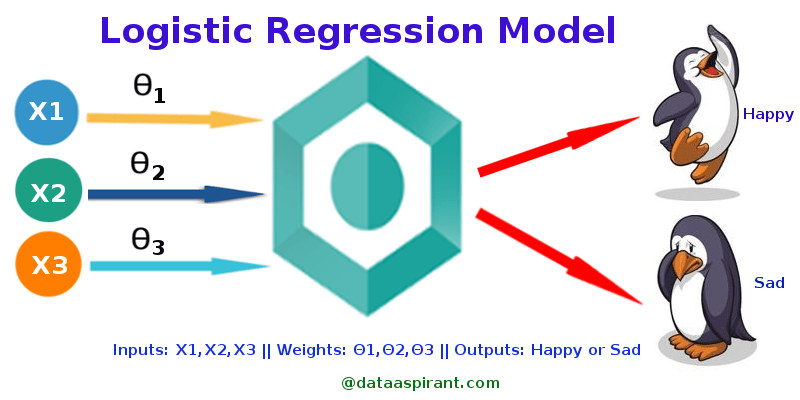
Logistic regression is one of the most popular algorithms for classification problems. It is called regression even though it is not a regression algorithm because the underlying technology is similar to Linear Regression. The term “logistic” comes from the statistical model used (logit model).
As seen in earlier releases, classification algorithms are used to classify the dataset into various classes; based on that, logistic classification is a type of binary classification.
Logistic regression is an extension of the linear regression model. Even though linear regression is good for regression, it does not work well for classification because the linear model doesn’t output probabilities and treats them as either 0 or 1 (Class A or Class B). Using this, it fits the dataset in a plane with each row as its point, then attempts to find the line that minimizes the distances between points and the plan.
Using the information given, the linear model will try to force a weird structure between the independent and the dependent variables.
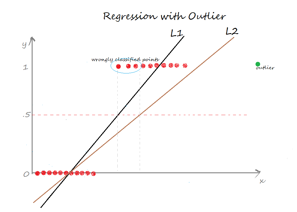
The line L1 is the best fit line when only the red points are considered, and it classified points to the right of the line as 1 and left as 0, which provides a decent indication of the data for classification even though there are a lot of wrongly classified points.
Now, if there is one point that is an extreme case (also called outlier), the best fit line transforms to L2, which is now classifying more points incorrectly to the extent where all the points that should be classified as 1 are 0. This drastic difference came just because of a single outlier.
Seeing such conditions, modifications were made to the linear regression algorithm, creating the famous logistic regression.
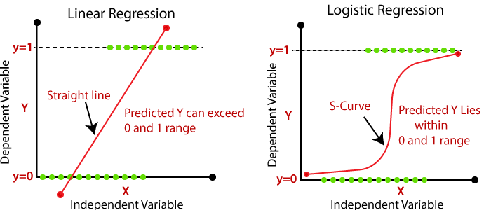
Instead of using a straight line in the plane logistic regression model uses the logistic function to fit the output of a linear equation between 0 and 1. Looking at the above diagram, it is evident that the S-curve created by logistic regression relates closely to the data points.
Logistic function:
When drawn on a 2-D plane, it looks like this:
In the places where X( independent variable) goes to infinity, Y (Dependent variable) goes to 1 and where X goes to negative of infinity, Y goes to 0.
This logistic function is also called a sigmoid function. It will take any real number and convert it into a probability between 0 and 1, hence great for binary classification.
Till now, there was only one independent variable (X) what will happen in a condition where there is more than one independent variable?
Then the linear equation will switch into
Here x1, x2,…. xp are all independent variables. The β values are calculated using the maximum likelihood estimation. This method checks the values of β through multiple iterations and finds the best fit of log odds, producing a likelihood function. Logistic regression works when this function is maximized, and the optimal values for the coefficients are found and then used in the sigmoid function to find the probability.
The blue line here is y=0.5, above which all points will be classified as class 1, and below it are class 0.
The probabilities found by the aforementioned formula are used here.
p≥0.5,class=1
p<0.5,class=0
So, the good thing about the logistic regression algorithm is that it not only classifies but also provides the probabilities. Knowing that a condition has a 90+% probability for a class compared to one with 51% is a big advantage.
The cost function of Logistic regression:
The cost function is a function that helps us understand how well the machine learning model works. It in itself calculates the difference between the actual and the predicted values and measures how wrong the algorithm was in prediction. By minimizing the value of the cost function most optimized result is found.
In logistic regression, the Log loss function is used.
Log Loss function:
Mathematically the log loss function is the average of the negative average of the log of corrected predicted probabilities for each instance.
By default, logistic regression gives probabilities with respect to the hypothesis.
For example, the hypothesis is “Probability that a person sleeps more than 10 hours a day.”
Here 1 represents a person sleeping more than 10 hours a day, and 0 is less than 10 hours.
| ID | Class | Probability |
| 1 | 1 | 0.93 |
| 2 | 1 | 0.76 |
| 3 | 0 | 0.2 |
| 4 | 0 | 0.4 |
| 5 | 1 | 0.78 |
Probability refers to the probability of the class being 1, i.e., the probability the person sleeps more than 10 hours a day.
For ID 3 and 4, we assign probabilities of 0.2 and 0.4, respectively, to represent their likelihood of belonging to their respective classes. In these cases, we use corrective probabilities, where the corrected probability for class 0 equals (1 – actual probability).
| ID | Class | Probability | Corrected Probability |
| 1 | 1 | 0.93 | 0,93 |
| 2 | 1 | 0.76 | 0.76 |
| 3 | 0 | 0.2 | 0.8 |
| 4 | 0 | 0.4 | 0.6 |
| 5 | 1 | 0.78 | 0.12 |
Now it’s time to find the Log of the correct probabilities:
| ID | Class | Probability | Corrected Probability | Log |
| 1 | 1 | 0.93 | 0.93 | -0.0315 |
| 2 | 1 | 0.76 | 0.76 | -0.1192 |
| 3 | 0 | 0.2 | 0.8 | -0.0969 |
| 4 | 0 | 0.4 | 0.6 | -0.2218 |
| 5 | 1 | 0.78 | 0.78 | -0.1079 |
Since the log for numbers, less than 1 is negative to deal with; this negative average is taken.
Thus the final formula becomes:
To summarise, the steps for the log loss function are:
- Find corrected probability
- Take the log of corrected probabilities
- Convert to the negative average of the values
The following code is for Logistic regression using Sklearn Library.
Loan Status Prediction:
As usual, let’s start with importing the libraries and then reading the dataset:
| import numpy as np import pandas as pd from sklearn.model_selection import train_test_split continue these codes now:from sklearn.linear_model import LogisticRegression from sklearn.metrics import accuracy_score |
| loan_dataset= pd.read_csv(‘../input/loan-predication/train_u6lujuX_CVtuZ9i (1).csv’) |
This dataset requires some preprocessing because it contains words instead of numbers and some null values.
| # dropping the missing values loan_dataset = loan_dataset.dropna() # numbering the labels loan_dataset.replace({“Loan_Status”:{‘N’:0,’Y’:1}},inplace=True) # replacing the value of 3+ to 4 loan_dataset = loan_dataset.replace(to_replace=’3+’, value=4) # convert categorical columns to numerical values loan_dataset.replace({‘Married’:{‘No’:0,’Yes’:1},’Gender’:{‘Male’:1,’Female’:0},’Self_Employed’:{‘No’:0,’Yes’:1}, ‘Property_Area’:{‘Rural’:0,’Semiurban’:1,’Urban’:2},’Education’:{‘Graduate’:1,’Not Graduate’:0}},inplace=True) |
In the first line, NULL values were dropped, then the Y and N (representing Yes and No ) in the dataset were replaced by 0 and 1; similarly, other categorical values are also given numbers.
| # separating the data and label X = loan_dataset.drop(columns=[‘Loan_ID’,’Loan_Status’],axis=1) Y = loan_dataset[‘Loan_Status’] X_train, X_test,Y_train,Y_test = train_test_split(X,Y,test_size=0.25,random_state=2) |
In the code, you can divide the dataset into training and testing sets, with the parameter test_size=0.25 indicating that you can use 25% of the data for testing, and the remaining 75% you can use it for training.
| model = LogisticRegression() model.fit(X_train, Y_train) |
Sklearn makes it very easy to train the model. You only need one line of code to accomplish this task.
Evaluating the model:
| X_train_prediction = model.predict(X_train) training_data_accuracy = accuracy_score(X_train_prediction, Y_train) |
This shows that the accuracy of the training data is 82%
| X_test_prediction = model.predict(X_test) test_data_accuracy = accuracy_score(X_test_prediction, Y_test) |
This shows that the accuracy of the training data is 78.3%
| input_data= (1,1,0,1,0,3033,1459.0,94.0,360.0,1.0,2)
# changing the input_data to a numpy array # reshape the np array as we are predicting for one instance prediction = model.predict(input_data_reshaped) |
The trained model will predict whether the loan is approved or not when you input random data into it.
Without Sklearn, Logistic Regression behaves similarly to a neural network, requiring both forward and backward propagation of the Loss function to optimize weights and biases.
Logistic Regression is a popular algorithm in machine learning, often used for binary classification problems. It is particularly effective when the outcome variable is categorical and has two classes. In this article, we will explore various aspects of Logistic Regression, including the sigmoid function, cost function, gradient descent, training and optimization, evaluation metrics, regularization techniques, handling imbalanced data, and extending it to multiclass classification scenarios.
I. Sigmoid Function: Activation for Binary Classification
The sigmoid function, also known as the logistic function, is a key component of Logistic Regression. It maps any real-valued number to a value between 0 and 1, making it suitable for binary classification. You can define the sigmoid function as:
sigmoid(z) = 1 / (1 + e^(-z))
Here, ‘z’ represents the linear combination of input features and their respective weights. The sigmoid function transforms the linear output into a probability value, indicating the likelihood of belonging to the positive class.
II. Cost Function and Gradient Descent in Logistic Regression
The cost function in Logistic Regression measures the discrepancy between the predicted probabilities and the actual labels. The most common cost function is the log-loss or binary cross-entropy function. You can define it as:
cost(h(x), y) = -y * log(h(x)) - (1 - y) * log(1 - h(x))
Here, ‘h(x)’ represents the predicted probability, and ‘y’ represents the actual label. The goal is to minimize this cost function.
Gradient descent is an optimization algorithm that iteratively adjusts weights to find the optimal set that minimizes the cost function. It moves in the opposite direction of the cost function’s gradient until reaching convergence.
III. Training and Optimization of Logistic Regression Model
To train a Logistic Regression model, we initialize the weights with random values. We then use gradient descent to update the weights iteratively, minimizing the cost function. The learning rate, which determines the step size during each iteration, plays a crucial role in the convergence of the algorithm.
IV. Evaluation Metrics for Logistic Regression
To evaluate the performance of a Logistic Regression model, you can use various metrics. Common evaluation metrics include accuracy, precision, recall, F1-score, and area under the ROC curve (AUC-ROC). These metrics provide insights into the model’s performance in terms of correctly predicting positive and negative classes.
V. Regularization Techniques in Logistic Regression
Regularization techniques, such as L1 and L2 regularization, help prevent overfitting in Logistic Regression models. These techniques add a regularization term to the cost function, which penalizes large weights. By controlling the regularization parameter, we can adjust the trade-off between model complexity and fitting the training data.
VI. Handling Imbalanced Data in Logistic Regression
Imbalanced datasets, where the number of samples in one class is significantly higher or lower than the other, can lead to biased models. To address class imbalance and enhance the performance of Logistic Regression on imbalanced datasets, one can employ various techniques such as oversampling, undersampling, and the synthetic minority oversampling technique (SMOTE).
VII. Multiclass Logistic Regression
While you can use Logistic Regression for binary classification, you can extend to handle multiclass classification problems using one-vs-rest or multinomial logistic regression. These approaches allow the model to handle more than two classes by training multiple binary logistic regression models or a single multiclass logistic regression model.
In conclusion, Logistic Regression is a powerful and interpretable algorithm for binary classification. Understanding the sigmoid function, cost function, gradient descent, training, evaluation metrics, regularization techniques, handling imbalanced data, and multiclass extensions provides a comprehensive understanding of this versatile algorithm. By mastering these concepts, you can effectively apply Logistic Regression to a wide range of real-world problems.
FAQs
What is Logistic Regression?
Logistic Regression is a statistical method used for binary classification, where the output variable is categorical and has only two possible outcomes.
How does Logistic Regression work?
Logistic Regression models the probability that an instance belongs to a particular class using the logistic function, which maps input features to probabilities between 0 and 1.
When should I use Logistic Regression?
Logistic Regression is suitable when dealing with binary classification problems, such as predicting whether an email is spam or not, based on features like sender, subject, and content.
What is the difference between Logistic Regression and Linear Regression?
Linear Regression predicts continuous outcomes, while Logistic Regression predicts probabilities. Additionally, Linear Regression uses a straight line to fit the data, while Logistic Regression uses the logistic function to produce an S-shaped curve.
How are the coefficients determined in Logistic Regression?
The coefficients (weights) are estimated using optimization algorithms like gradient descent, which minimize a cost function such as the binary cross-entropy loss.
Can Logistic Regression handle multi-class classification?
Yes, Logistic Regression can be extended to handle multi-class classification using techniques like one-vs-rest or multinomial Logistic Regression.
What are the assumptions of Logistic Regression?
The key assumptions include linearity between the log odds of the outcome and the predictors, independence of observations, absence of multicollinearity, and a large sample size for stable parameter estimates.