
Naive Bayes is a classification algorithm which checks the probability of a test point belonging to a class. Unlike other algorithms, Naive Bayes is purely a classification algorithm.
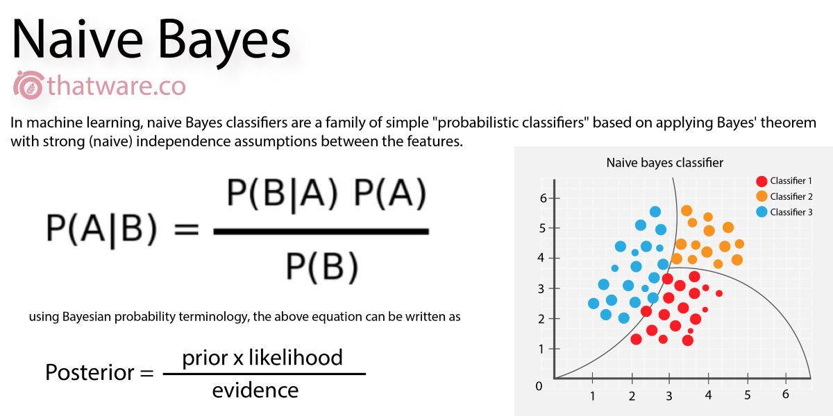
As explained in the last release this is the formula for the Bayes theorem and as the algorithm name suggests Naive Bayes is inspired by the Bayes theorem.
Naive Bayes is not one algorithm it is a family of algorithms following the assumption no two variables are dependent on each other.
For example, A car may be red and seat 2 people. These are 2 independent variables and can be used in the Naive Bayes algorithm to differentiate between a honda and a Ferrari.
This condition of independence becomes one drawback for the algorithm because in real life most features are interrelated.
Naive Bayes works well for large datasets and its simplicity outperforms most classification methods.
The main advantages are:
- It is fast, and easy to understand
- It is not prone to overfitting
- It does not need much training data
There are different types of Naive Bayes classifiers and the 3 major types are:
- Bernoulli Naive Bayes: This is the case when there are only 2 classes. Options like “Yes” or “No”, “True” or “False” etc. Data follows the Bernoulli distribution hence the name.
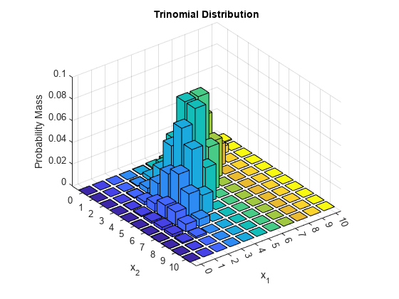
- Multinomial Naive Bayes: This type follows the multinomial distribution where events are represented by feature vectors. This is usually used in natural language processing to tag emails and documents into various categories.
- Gaussian Naive Bayes: This is the type where numerical and continuous features are present. The probabilities are calculated using the Gaussian distribution. This is also used for text classification in natural language processing where the probability of appearance of words is used to tag the texts.
Gaussian Distribution Graph
A majority of research papers on text classification start off by using the Naive Bayes classifier as the baseline model.
Now that there is an introductory idea of how Naive Bayes works let’s dive a little more into the maths behind it.
Starting with the Bayes theorem
Here X represents the independent variables while y represents the output or dependent variable.
The assumption works that all variables are completely independent of each other hence X translates to x1, x2 x3 and so on
So, the proportionality becomes
Combining this for all x
Now the target for the Naive Bayes algorithm is to find the class which has maximum probability for the target. Which refers to finding the maximum value of y
For this argmax operation is used.
Python Implementation for Naive Bayes
Link to run and check code:
Importing the libraries
| import pandas as pd import numpy as np from sklearn.naive_bayes import GaussianNB |
Reading the dataset
| dataframe = pd.read_csv(“../input/titanic/train.csv”) |
Taking only the independent and useful data into the final data frame
| # Name, Ticket , Passanger ID have almost no correlation to the outcome
final_dataframe= dataframe[[‘Survived’, ‘Pclass’, ‘Sex’, ‘Age’, ‘SibSp’, |
Labeling the values in the “Sex” column of the dataset to numbers
| final_dataframe[“Sex”] = final_dataframe[“Sex”].replace(to_replace=final_dataframe[“Sex”].unique(), value = [1 , 0]) |
One hot encoding the dataset
This is an encoding algorithm in the sklearn library to get categorical data into various columns and make encode it in a way that the dataset can be sent to the machine learning model
| # One hot encoding final_dataframe = pd.get_dummies(final_dataframe, drop_first=True) |
Creating the training and testing datasets
| train_y = final_dataframe[“Survived”] train_x = final_dataframe[[‘Pclass’, ‘Sex’, ‘Age’, ‘SibSp’, ‘Parch’, ‘Fare’, ‘Embarked_Q’,’Embarked_S’]] |
Train Test Split for the data
| from sklearn.model_selection import train_test_split
train_data, val_data, train_target, val_target = train_test_split(train_x,train_y, train_size=0.8) |
Fighting the dataset into the model and then using it to predict the test dataset.
| model = GaussianNB() model.fit(train_data,train_target) val_pred= model.predict(val_data) |
Calculating Accuracy
| from sklearn.metrics import accuracy_score
print(‘Model accuracy score: {0:0.4f}’. format(accuracy_score(val_target, val_pred))) |
This was a sample for the famous Titanic dataset where Naive Bayes is used with an accuracy of 76.9%
Things that can be done for better usage of the Naive Bayes Model:
- Transform continuous data into Gaussian distribution if it is not already in it.
- When needed, apply smoothing techniques like Laplace Correction before the prediction of class in the test dataset.
- Remove the interdependent features.
- Ensembling techniques like bagging and boosting are not applicable for Naive Bayes because these methods work with variance minimization, and Naive Bayes has no variance to minimize.
Naive Bayes is a popular and simple classification algorithm based on Bayes’ theorem and the assumption of feature independence. It is widely used in text classification, spam filtering, sentiment analysis, and other applications where quick and efficient classification is required. Despite its “naive” assumption, Naive Bayes often performs well and can be a powerful tool in machine learning.
The algorithm works as follows:
- Dataset Preparation: To apply the Naive Bayes algorithm, a labeled dataset is required. Each data point consists of a set of features and a corresponding class label. The features can be categorical or continuous, but they need to be converted into discrete values for categorical features or into bins for continuous features.
- Feature Independence Assumption: The Naive Bayes algorithm assumes that the features are conditionally independent given the class variable. This assumption simplifies the calculation of probabilities by treating each feature independently. Although this assumption is rarely true in real-world data, Naive Bayes can still provide reasonable results in many cases.
- Calculating Class Probabilities: Naive Bayes starts by calculating the prior probabilities of each class in the training dataset. The prior probability represents the probability of each class occurring without considering any features. It is calculated by dividing the number of data points in each class by the total number of data points.
Some more points to consider:
- Calculating Feature Probabilities: For each feature and class combination, Naive Bayes calculates the conditional probability. This probability represents the likelihood of a feature’s value given a specific class. The conditional probability is estimated by counting the occurrences of each feature value within each class and dividing by the total count of that class.
- Combining Feature Probabilities: To make a prediction for a new data point, Naive Bayes combines the probabilities of all features given a specific class. This is done by multiplying the conditional probabilities of each feature value. In some cases, a log transformation is applied to avoid numerical underflow.
- Choosing the Maximum Probability: After calculating the probabilities for each class, Naive Bayes selects the class with the highest probability as the predicted class for the new data point.
- Laplace Smoothing: In cases where a feature value is not present in the training data for a particular class, the conditional probability becomes zero. To avoid zero probabilities and prevent the algorithm from assigning zero likelihood to unseen data, Laplace smoothing (also known as additive smoothing) is often applied. This involves adding a small value (usually 1) to the numerator and adjusting the denominator accordingly to smooth out the probability estimates.
Naive Bayes offers several advantages:
- Simplicity: Naive Bayes is simple to understand and implement. Its straightforward probabilistic approach makes it accessible to beginners in machine learning.
- Fast and Efficient: Naive Bayes is computationally efficient, especially for large datasets. The algorithm’s simplicity allows it to process data quickly, making it suitable for real-time or high-volume applications.
- Handles Irrelevant Features: Naive Bayes can handle irrelevant or redundant features without significantly impacting its performance. Since it assumes feature independence, irrelevant features do not affect the probability calculations.
- Works Well with High-Dimensional Data: Naive Bayes performs well even when the number of features is high. It is not as affected by the curse of dimensionality as other algorithms.
However, Naive Bayes has limitations:
- Assumption of Feature Independence: The assumption of feature independence might not hold true in many real-world datasets. If the features are highly correlated, Naive Bayes may produce suboptimal results.
- Limited Expressive Power: Naive Bayes has limited expressive power compared to more complex algorithms. It may struggle with complex relationships and interactions between features.
- Sensitivity to Feature Distribution: While Naive Bayes assumes conditional independence of features given the class, it does not consider the actual distribution of the features. If the feature distribution significantly deviates from the assumption, Naive Bayes may not perform well.
In conclusion, Naive Bayes is a simple yet powerful classification algorithm based on Bayes’ theorem. Despite its assumption of feature independence, it often performs well in various applications. Its speed, efficiency, and ability to handle high-dimensional data make it a popular choice for text classification and other classification tasks. While it has its limitations, Naive Bayes provides a valuable tool for quick and efficient classification in many machine-learning scenarios.
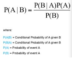
Conditional probability is a fundamental concept in probability theory that measures the probability of an event occurring given that another event has already occurred. It provides a way to analyze and quantify the relationship between events, taking into account additional information or conditions.
We denote the conditional probability of event A given event B as \(P(A|B)\) and calculate it using the formula::
P(A|B) = P(A ∩ B) / P(B)
where P(A ∩ B) represents the probability of both events A and B occurring simultaneously, and P(B) is the probability of event B occurring.
Conditional probability allows us to update our knowledge or beliefs about the occurrence of an event based on new information. It helps us understand how the likelihood of an event changes when we have additional context.
For example, let’s consider a standard deck of 52 playing cards. Suppose we draw a card at random and want to find the probability of drawing an ace from the deck. The probability of drawing an ace is 4/52 since there are four aces in the deck.
Now, let’s say we know that the drawn card is a spade. We want to find the probability of drawing an ace given that the card is a spade. We now have additional information or a condition, which is that the card is a spade.
What’s more to look at?
Since there are 13 spades in the deck (including the four aces), the probability of drawing a spade is 13/52. Now, out of these 13 spades, there are four aces. Therefore, the probability of drawing an ace given that the card is a spade is 4/13. This is an example of conditional probability, where the probability of drawing an ace changes based on the condition that the card is a spade.
Conditional probability allows us to make more informed decisions and predictions by incorporating relevant information. You can use it in various fields, including statistics, machine learning, finance, and genetics, to analyze and model complex relationships between variables.
Conditional probability also plays a crucial role in Bayes’ theorem, a fundamental concept in probability theory and statistics. Bayes’ theorem allows us to update our beliefs about the probability of an event based on new evidence or observations.
Bayes’ theorem states:
P(A|B) = (P(B|A) * P(A)) / P(B)
In this equation, P(A) and P(B) represent the independent probabilities of events A and B occurring, respectively, while P(B|A) denotes the conditional probability of event B occurring given that event A has occurred.
Bayes’ theorem provides a framework for incorporating new information or data to update our prior beliefs or probabilities. It has widespread applications in fields such as medical diagnosis, spam filtering, and pattern recognition.
Understanding conditional probability is essential for interpreting statistical analyses, making informed decisions, and developing accurate predictive models. It allows us to reason about events in a probabilistic framework, taking into account additional information and conditions that influence the likelihood of an event.
In conclusion, conditional probability is a fundamental concept in probability theory that measures the likelihood of an event occurring given that another event has already occurred. It provides a way to incorporate additional information or conditions to update our beliefs about the occurrence of an event. Conditional probability plays a crucial role in various fields and serves as a foundational element of Bayes’ theorem. Bayes’ theorem provides a framework for updating probabilities as new evidence becomes available. Understanding conditional probability is essential for probabilistic reasoning, statistical analysis, and decision-making.
FAQs
What is Naive Bayes?
Naive Bayes is a probabilistic machine learning algorithm used for classification tasks, based on Bayes’ theorem.
How does Naive Bayes work?
Naive Bayes calculates the probability of each class given the input features and selects the class with the highest probability as the prediction. It assumes independence between features, hence the term “naive.”
When should I use Naive Bayes?
Naive Bayes is suitable for classification tasks, especially when working with text data, such as email spam detection or document classification.
What makes Naive Bayes “naive”?
Naive Bayes assumes that all features are independent of each other, which is often not true in real-world datasets. Despite this simplifying assumption, Naive Bayes can perform well in practice, especially with large datasets.
Can Naive Bayes handle continuous and categorical features?
Yes, Naive Bayes can handle both continuous and categorical features by applying different probability distributions such as Gaussian for continuous and multinomial or Bernoulli for categorical features.
How does Naive Bayes handle missing data?
Naive Bayes can handle missing data by ignoring the missing values during probability calculation or using techniques like mean or median imputation.
Is Naive Bayes affected by imbalanced datasets?
Naive Bayes can be affected by imbalanced datasets, as it may produce biased predictions towards the majority class. Techniques like oversampling, undersampling, or adjusting class priors can help address this issue.