Classification algorithms depend on the dataset being used, and data scientists have curated various algorithms that can be used in certain situations.
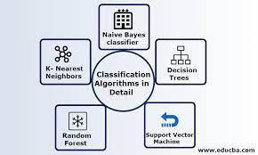
Most popular types of Classification Algorithms:
- Linear Classifiers
- Logistic regression
- Naive Bayes classifier
- Support vector machines
- Kernel estimation
- k-nearest neighbor
- Decision trees
- Random forests
Let’s discuss this in more detail and understand when to use which algorithm.
Linear Classifiers:
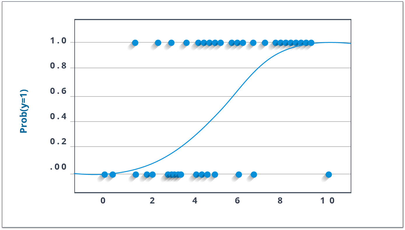
1. Logistic Regression:
Even though the term Regression is used in the name, it is not a regression algorithm but a classification one. This algorithm gives us a binary output of 0 or 1, pass or fail, etc.
The logistic regression algorithm fits the dataset into a function and then predicts the probability of the output being 0 or 1.
Probability is given by P(Y=1|X) or P(Y=0|X). This represents the probability of 1 when X has occurred and the probability of 0 when X has occurred.
Here X represents the independent variables, and Y represents the dependent variables.
This algorithm can calculate the probability of a situation between 0 and 1 or determine whether an object is in the picture.
2 important parts of the logistic regression algorithm are the hypothesis and sigmoid curve, which will be discussed later.
2. Naive Bayes:
Naive Bayes is not one algorithm it is a family of algorithms following the same assumptions, such as no two variables are dependent on each other, and the algorithm follows the Bayes theorem.
For example, A car may be red and seat 2 people. These are 2 independent variables and can be used in the Naive Bayes algorithm to differentiate between a honda and a Ferrari.
Bayes theorem formula:
Where:
P(A|B) – the probability of event A occurring, given event B has occurred
P(B|A) – the probability of event B occurring, given event A has occurred
P(A) – the probability of event A
P(B) – the probability of event B
Naive Bayes is mainly used for text classification problems and multiclass problems. It is a quick way to predict categories even when the dataset is small.
The biggest drawback is the assumption that all data in the dataset should be independent. In real-life data, this is very difficult to follow. Also, if a category was not present in the training dataset, then the model will give a probability of 0 and not make any prediction.
Support Vector Machine Algorithm:
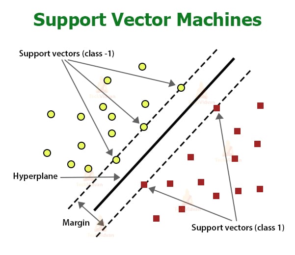
The SVM algorithm plots the categories on an n-dimensional plane (n is the number of independent variables). Then SVM algorithm creates decision boundaries to separate them into categories/classes. The best decision boundary is the hyperplane. The algorithm chooses the extreme data points to create such a hyperplane. These data points are called support vectors, hence the name of the algorithm Support Vector Machines.
The image below represents a 2-dimensional SVM model dividing the datasets into 2 categories.
SVM algorithm is most used for Face detection, image classification, text categorization, etc.
K-Nearest Neighbour
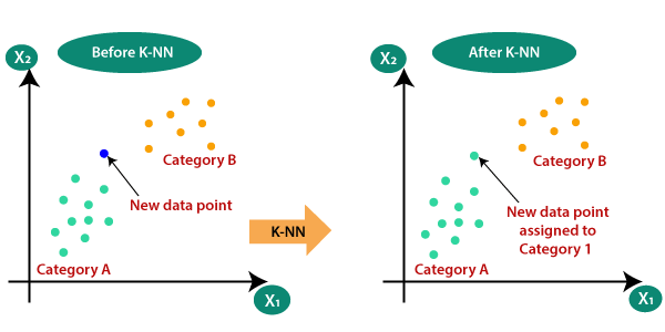
K_nearest neighbor (KNN) is one of the most basic classification algorithms. It follows the assumption that similar things exist in close proximity to each other.
The K-nearest neighbor algorithm calculates the distance between the various points whose category is known and then selects the shortest distance for the new data point.
This is an amazing algorithm when working with small datasets, and it is so simple that it doesn’t require additional assumptions or tuning.
The most famous use-case for KNN is in the recommender systems, such as recommending products on Amazon, movies on Netflix, or videos on Youtube. KNN may not be the most efficient approach for large amounts of data, so companies may use their algorithms to do the job, but for small-scale recommendation systems, KNN is a good choice.
Decision Trees
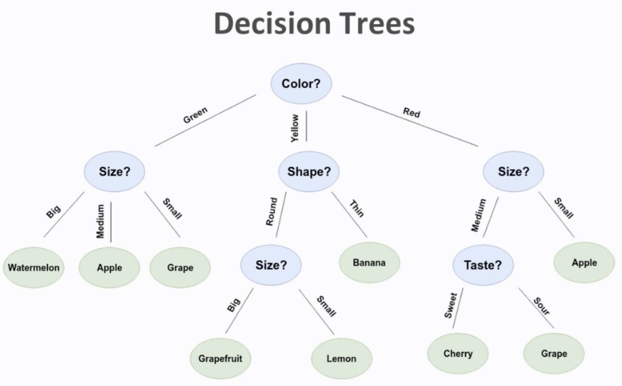
The Decision Tree algorithm uses a tree-like representation to solve problems. It starts by splitting the dataset into 2 or more sets by using the rules found in the dataset. Each decision node asks a question to the dataset and then sorts it accordingly until it reaches the desired categories. This last layer of nodes is called the leaf nodes.
Let’s use this example where fruits need to be classified. The root node starts with a color, sorting the dataset into Green, Yellow, and Red. Then it checks the size of the Red and Green datasets while checking the shape of the yellow part. The ones coming from the root node’s Yellow, Green, and Red sides have been classified in the next step into Banana, watermelon, Apple and Grape. These parts of the dataset have gotten the label they needed. Next, it takes another iteration for the still unclassified data. It divides the yellow side by size into grapefruit and lemon while going for taste in the red size and dividing into cherry and grape.
In the end, the leaf nodes can be seen with the classifier’s outputs, i.e., Watermellon, Apple, Grape, Grapefruit, Lemon, Banana, and Cherry.
Random Forest Algorithm
At the time of training, Random forest constructs a bunch of decision trees to help get the output category/class. This algorithm helps prevent overfitting and is more accurate than simple decision trees in most cases.
Since it uses more than one decision tree, the algorithm’s complexity increases, real-time prediction becomes slow, and it does not provide good results when data is sparse.
One use case of this algorithm is in the healthcare industry, where it is used to diagnose patients based on past medical records. It can also be used in the banking industry to detect the creditworthiness of loan applicants.
This was to give an introductory intuition to the algorithms More details to follow.
In the field of machine learning, the choice of classifier plays a critical role in determining the success of a predictive model. There is no one-size-fits-all approach, as different classifiers have distinct strengths and weaknesses. In this article, we will delve into the various factors that necessitate the use of different types of classifiers, including the bias-variance tradeoff, complexity of classification problems, handling non-linearity in data, dealing with imbalanced data, interpretability and explainability, scalability and efficiency, robustness to noise and outliers, flexibility and adaptability to different data distributions, as well as case-specific requirements and constraints.
I. Bias-Variance Tradeoff and Model Selection
The bias-variance tradeoff is a fundamental concept in machine learning. Classifiers with high bias tend to oversimplify the underlying patterns, leading to underfitting, while those with high variance overfit the training data, resulting in poor generalization to unseen instances. Different types of classifiers have varying biases and variances, making it crucial to strike the right balance when selecting a model.
II. Complexity of Classification Problems
Classification problems can vary widely in terms of complexity. Some problems may exhibit simple linear decision boundaries, while others require more complex non-linear relationships to be captured. Different classifiers offer varying degrees of flexibility in handling complex patterns, making it necessary to choose an appropriate classifier based on the complexity of the problem at hand.
III. Handling Non-Linearity in Data
Many real-world datasets exhibit non-linear relationships between features and the target variable. Linear classifiers may struggle to capture such non-linearities effectively. Non-linear classifiers, such as support vector machines with kernel methods or decision trees, can better model intricate patterns, making them essential for accurately classifying non-linear data.
IV. Dealing with Imbalanced Data
Imbalanced datasets, where the number of instances in different classes is uneven, pose a challenge for classifiers. Some classes may be underrepresented, leading to biased models that favor the majority class. Specialized classifiers, like ensemble methods or those equipped with cost-sensitive learning, can handle imbalanced data and improve classification performance.
V. Interpretability and Explainability
In certain domains, interpretability and explainability of the classifier’s decision-making process are paramount. Linear classifiers, such as logistic regression or linear support vector machines, offer transparent models that allow for easy interpretation. In contrast, complex models like neural networks may provide high accuracy but lack interpretability, making it necessary to consider the tradeoff between interpretability and performance.
VI. Scalability and Efficiency
The scalability and efficiency of classifiers become critical when dealing with large-scale datasets or real-time applications. Some classifiers, like k-nearest neighbors or linear classifiers, have low computational complexity and can handle large datasets efficiently. On the other hand, complex models like deep neural networks may require significant computational resources, making them less practical for resource-constrained environments.
VII. Robustness to Noise and Outliers
Real-world datasets are often contaminated with noise and outliers, which can adversely impact classification performance. Robust classifiers, such as support vector machines or decision trees with pruning, can handle noisy data more effectively and provide better robustness against outliers.
VIII. Flexibility and Adaptability to Different Data Distributions
Data distributions can vary significantly across different domains and applications. Certain classifiers, like Naive Bayes or Gaussian processes, make specific assumptions about the data distribution and may perform well under certain conditions. However, more flexible classifiers, such as random forests or gradient boosting, can adapt to diverse data distributions and offer improved performance across a wide range of scenarios.
IX. Case-Specific Requirements and Constraints
Lastly, the choice of classifier may be driven by specific requirements and constraints of the problem at hand. For instance, in medical applications, classifiers with high sensitivity (recall) may be crucial for correctly identifying rare diseases. In legal or regulatory contexts, classifiers that adhere to certain fairness or non-discrimination constraints may be necessary.
In conclusion, the need for different types of classifiers arises due to a variety of factors such as the bias-variance tradeoff, complexity of classification problems, non-linearity in data, imbalanced data, interpretability and explainability requirements, scalability and efficiency considerations, robustness to noise and outliers, adaptability to different data distributions, as well as case-specific requirements and constraints. By understanding these factors and selecting the appropriate classifier accordingly, practitioners can build more accurate and robust classification models tailored to the specific needs of their applications.
FAQs
Why do we need different types of classifiers?
Different classifiers excel in different scenarios due to their unique characteristics, making it essential to have a variety of options to suit diverse datasets and problem types.
How does the choice of classifier impact model performance?
The choice of classifier can significantly impact model performance, as certain algorithms may better capture the underlying patterns in the data or handle specific challenges such as high dimensionality or class imbalance.
What factors should be considered when selecting a classifier?
Factors to consider include the nature of the data (linear vs. non-linear relationships), dataset size, interpretability of the model, computational resources, and the desired balance between bias and variance.
Can you provide examples of scenarios where different classifiers are preferred?
For instance, decision trees are suitable for interpretable models and handling non-linear relationships, while support vector machines (SVM) excel in high-dimensional spaces and scenarios with clear margins of separation.
How do ensemble methods address the limitations of individual classifiers?
Ensemble methods combine multiple classifiers to improve overall performance by leveraging the strengths of each individual classifier and mitigating their weaknesses, leading to more robust predictions.
Are there classifiers specifically designed for handling imbalanced datasets?
Yes, classifiers like Random Forest and Gradient Boosting Machines (GBM) are known to perform well on imbalanced datasets by adjusting class weights or using techniques like bagging and boosting to address class imbalance.
Can the choice of classifier affect the interpretability of the model?
Yes, some classifiers such as decision trees and logistic regression produce interpretable models with easily understandable rules, while others like neural networks and support vector machines may offer higher predictive accuracy at the cost of interpretability.