
Every Neural Network has 2 main parts
- Forward Propagation
- Backward Propagation
In this release, let’s take a deep dive into both these parts.
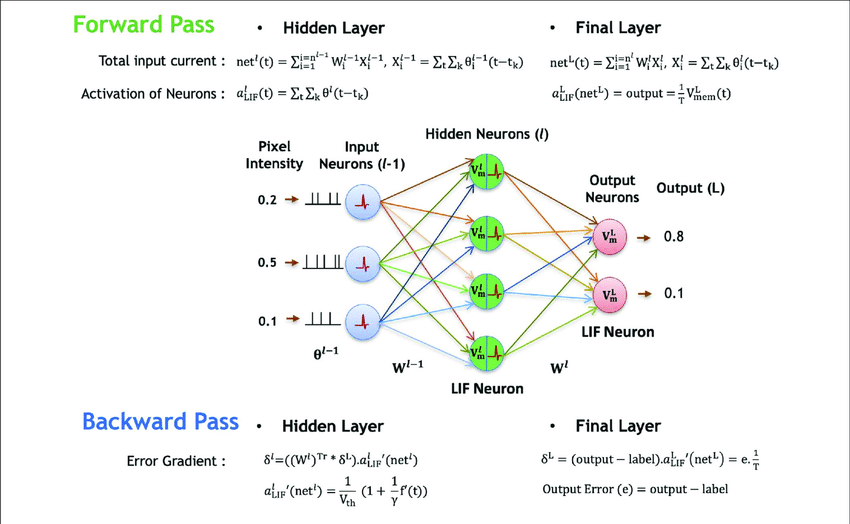
Forward Propagation
This refers to the calculation and storage of variables going from the input layer to the output layer.
Here the data flow via the hidden layers in the forward direction. Each layer accepts the input data, processes it as per the activation function and passes it to the next layer.
For a single layer, the propagation mathematically looks like
Prediction= A(A(XWh)Wo)
A= Activation function
Wh and Wo are the weights
X is the input.
Let us assume a ReLu activation function then the layer would look somewhere along the line of
| def relu(z): return max(0,z)def feed_forward(x, Wh, Wo): # Hidden layer Zh = x * Wh H = relu(Zh)# Output layer Zo = H * Wo output = relu(Zo) return output |
This simple method can be seen as a series of nested functions.
Here the input X receives weights and moves towards the Hidden Layers H1 and H2 from where weights are further added to it and sent towards the output layers O1 and O2.
Input Layer size = 1
Hidden Layer Size = 2
Output Layer Size = 2
Once all the hidden weights and biases are set it is time for the backward propagation to come into play and make sure it works with the least possible error.
In the previous single-layered forward propagation the weights were scalar numbers now they will become numpy arrays.
| def init_weights(): Wh = np.random.randn(INPUT_LAYER_SIZE, HIDDEN_LAYER_SIZE) * \ np.sqrt(2.0/INPUT_LAYER_SIZE) Wo = np.random.randn(HIDDEN_LAYER_SIZE, OUTPUT_LAYER_SIZE) * \ np.sqrt(2.0/HIDDEN_LAYER_SIZE) |
And the biases are
| def init_bias(): Bh = np.full((1, HIDDEN_LAYER_SIZE), 0.1) Bo = np.full((1, OUTPUT_LAYER_SIZE), 0.1) return Bh, Bo |
These weights and biases are added to the input in a manner same as the one for single-layered neurons.
Backward Propagation
Backpropagation is the fine-tuning of the weights based on the error rate (or loss) obtained in the previous iteration ( for the purpose of neural networks each iteration is called an epoch). Giving proper weights makes the model more reliable. Once forward propagation is over the algorithm present has a lot of loss and is not fine-tuned. Using optimization functions like gradient descent the weights are curated to give smaller loss in each epoch.
The cost in each step is calculated using derivatives of the cost function.
For a 10-layered neural network, it looks something like
Instead of calculating all derivatives in every step the chain rule is used where the previous derivative is memorised and used in the next step. In each layer, the error is calculated and the error is the derivative of the cost function.
For a case with ReLu activation function and mean squared cost function the code looks something like this.
| def relu_prime(z): if z > 0: return 1 return 0def cost(yHat, y): return 0.5 * (yHat – y)**2def cost_prime(yHat, y): return yHat – y def backprop(x, y, Wh, Wo, lr): # Layer Error # Cost derivative for weights # Update weights |
Here the maths behind each function is:
To summarize:
Using the input variables x and y, the forward pass or propagation calculates output z as a function of x and y i.e. f(x,y).
During backwards pass or propagation, on receiving dL/dz (the derivative of the total loss, L with respect to the output, z), we can calculate the individual gradients of x and y on the loss function by applying the chain rule