
The neural network algorithm is derived from the functioning of the human brain. It is composed of multiple neurons similar to the brain. Each neuron is made up of input, weight, activation function and output.
In every neuron, the weight acts as a guiding path for the algorithm that is over the algorithm the weight is constantly tweaked to improve the output. It varies as per the relative importance of different features.
So if we consider the output of a particular neuron we may get it as
Where represent the weight corresponding to the particular feature
denote the numerical input of every neuron and is the bias in each
is the non-linear function called the activation function. Its purpose is to introduce non-linearity. It also serves the purpose to map the output between 0 to 1.
In simpler words, the function’s sole purpose is to map the non-linear output to values between 0 and 1.
The training phase of ANN (Artificial neural network)
At the end of the day, we want our model to generate the best possible results. It achieves this by creating a probability-weighted association between inputs and outputs i.e. it takes an input and generates an output. It then compares the output with the expected result and calculates the error in the generated output.
Often, we use Mean Squared Error or MSE
Where denotes the total number of inputs is the expected output and is the neural network output.
The algorithm repeatedly calculates the error using a cost function and tries to minimize the cost function.
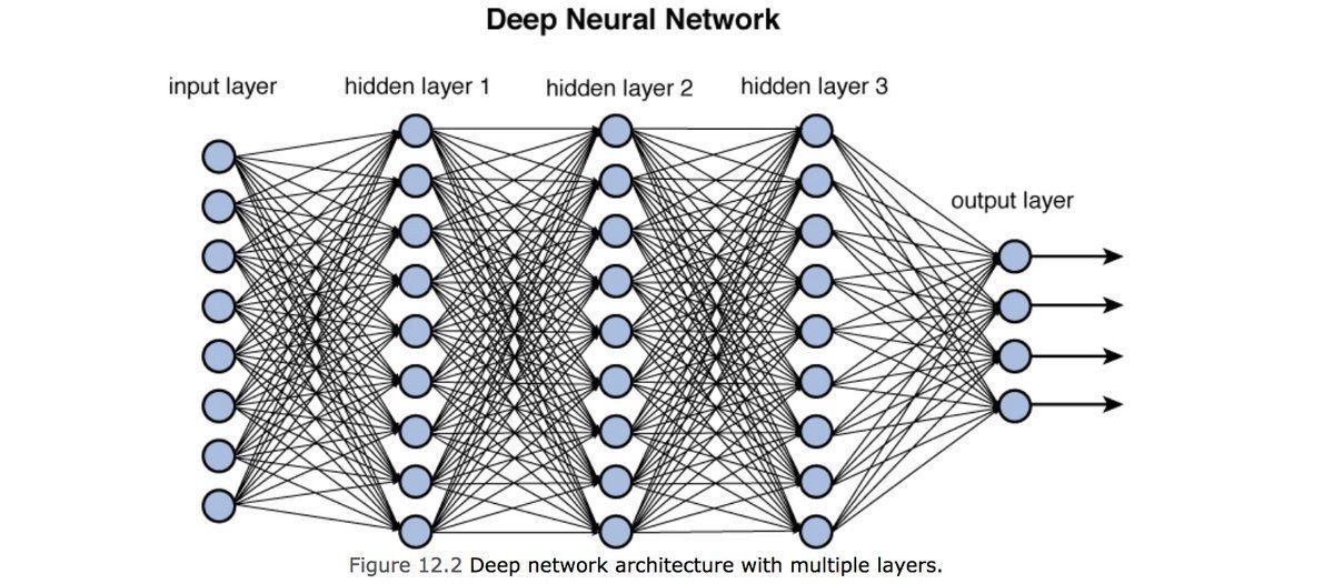
A typical neural network consists of input layers, hidden layers and an output layer.
So in a typical ANN, the input layer is just the data points, used to train the algorithm. The succeeding layers are called hidden layers. The final layer is the output layer. In the output layer, there is a node for each corresponding class of output. So when the algorithm proceeds forward it keeps on assigning value to each new node which acts as input to the next layer until it all converges into one of the classes in the output layer.
The learning process of ANN
ANN uses an iterative process to improve the output result. To achieve this it takes an input generating corresponding output. Then, the error is computed, and the algorithm processes the next set of data, using the error to readjust the weights assigned to various input features. Initially, random weights are assigned to these features. In the iterative process, the algorithm reprocesses the same inputs with the hope that the cost will be minimized, and the output will closely match the expected result. However, some networks may struggle to optimize the result, often due to insufficient data rather than a flaw in the algorithm’s design. Ideally, there should be ample data available for both training and validation purposes.
It helps in better understanding noisy data as well as being able to classify patterns on which they have not yet been trained. A commonly known ANN algorithm is Backpropagation.
Understanding ANN using Perceptron Algorithm
The Perceptron algorithm is considered one of the simplest algorithms in terms of ANN. It uses linear separation if there are 2 features to predict the output and corresponding hyperplane in higher dimensions.
It uses stochastic gradient descent. The model initially multiplies the provided inputs by the random weights. The weighted sum is then passed through a function that maps the output to a value between 0 and 1.
Data points from the dataset are fed into the model one by one. The model generates an output and then compares it to the expected output. This process is known as feed-forward. Next, you calculate the corresponding errors, which involves comparing the model’s output with the expected or original output. This value is then passed through the network, resulting in updates to the model’s weights or linear coefficients, as is the case with the perceptron algorithm. This is known as Back-Propagation.
Conclusion
In other words, Back-Propagation is a technique for training the weights of a multilayer feed-forward neural network. As a result, a network topology comprising one or more levels is necessary, with each layer being fully connected to the next. One input layer, one hidden layer, and one output layer constitute a general neural network. The process of updating the weights using backpropagation in the case of the perceptron algorithm is called the perceptron update rule. When you apply this update rule once for every data point in the training set, it’s referred to as an epoch.
The network’s initial weights are chosen randomly. Moreover, the data is shuffled and randomly split into training and testing sets. This randomization helps assess the algorithm’s effectiveness because its learning dataset varies with each run, resulting in different classification rates. To evaluate the algorithm’s performance, it’s essential to conduct repeated classifications and then calculate the average of all the classification accuracies.