
There are situations in daily life where we want to know the relationship between various factors, for example, if the price of petrol increases would it affect the sales of cars or does changing the location of the house will it affect the price. The process of finding this relationship between multitudes of factors is known as regression
in more formal words, regression refers to the study of the relationship between the variables so that one can predict the unknown value of one variable for a known value of another variable.
To better understand the regression, we need to be familiar with two terms
- Independent variable:- These refer to the factors or the variables based upon which the situation is analyzed. These variables don’t change and indicate details about the dependent variable.
- Dependent variable:- It refers to the result, i.e., the sales of cars or the house price. In formal terms, the factor is affected based on the independent variables.
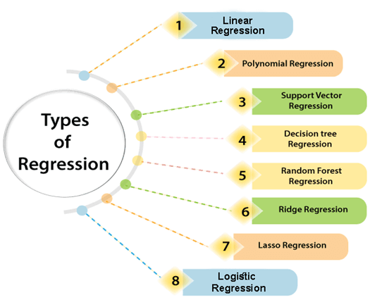
Types of regression
Image source https://static.javatpoint.com/tutorial/machine-learning/images/types-of-regression.png
So what is linear regression?
On a dataset, if the end goal is to find some linear relationship between the independent variable so that when an unknown point is given, a prediction can be made. In the case where there is only 1 independent feature, it is called Uni-variate linear regression, and if there are multiple features, it is called Multiple linear regression.
In the case of Univariate linear regression, a line is formed on a 2-D plane that shows the linear relationship between the independent and dependent variables. While in the case of multivariate linear regression, a hyperplane is formed.
A regression model tries to find a function that would suitably fit the training data and predict with accuracy the training data
In the case of linear regression, it is a linear function of the form:
- Where y denotes the predicted value (dependent variable)
- b is called the bias term or the offset
- Are called the modal parameters (these are the values that our modal tries to learn using the training data)
- are called the feature values (independent variables)
Understanding linear regression
To understand anything, the best way is to understand how it works under the hood let’s start by generating a random data set to test our linear regression algorithm.
| import numpy as np import matplotlib.pyplot as plt# generate random data-set np.random.seed(7) x = np.random.rand(100, 1) y = 15 + 2 * x + np.random.rand(100, 1)# plot plt.scatter(x,y,s=10) plt.xlabel(‘x’) plt.ylabel(‘y’) plt.show() |
The above code sets the random seed to 7 i.e., when the rand function of the numpy tries to generate random numbers, it will end up generating the same numbers on each iteration this is done to ensure the same values x
Next, let the value of y at each x be given by
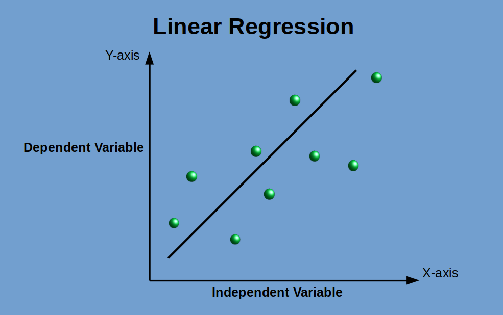
If we see the plot of the generated data, it looks like
So, intuitively the line which will distribute the data nearly accurately will look like something
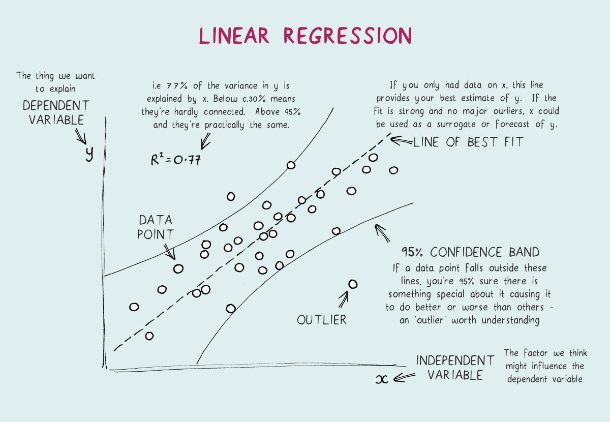
The line we just thought, i.e., which divides the data, is known as the best fit line.
How do we decide best-fit line?

What does the best fit line represent? It acts as the line which tells us for a particular value of x what might be the value of y.
So the best fit line is, and the regression model needs to calculate the value of m and c using the training data set.
But it is possible that the actual value of y might not be equal to the predicted value in that case the difference between the predicted value and the actual value is called residuals. So the best fit line is a line that divides the data into equal parts along with minimum residuals. The sum of all residuals is also called the cost function.
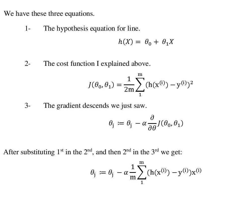
How to calculate the cost function?
Suppose we have a point xi, yi
And where denotes various features, so at first thought, we may think that Since the error is caused due to residuals, let’s add them
Since calculation for multi-feature would be complex, let us consider x to be with one feature, so our error becomes
This method is inaccurate because residuals on the opposite sides of the line cancel each other out.
Let’s take the absolute value of the error so our new function becomes
Consider another scenario
Let the best fit line shift a bit towards a point the error function will not change as the error is reduced in one term and increases in another to overcome this issue.
We must square the error function.
Consider the example; let the original errors be 2 and 2
Let after shifting new errors are 1 and 3
using the old formula, our error would be
Which is the same as the original error, but after
Change in the formula this change will affect the error as in the original case; it would become
whereas afterward, it will become
So our error function would be
but to find the best fit line, the error or cost function needs to be minimized, so,
differentiate cost function concerning m and c
So are final differentiation wrt to m will be
Upon dividing by the number of training samples, N
We get
Which is effectively the mean as one-dimensional data is taken for this case.
So, the cost function can be written as:
Similarly, differentiating concerning c
We get
Which can be re-written as
Again dividing by N
We get
So finally, we get both equations which are
Upon substituting the value of C in the first equation, we get
and
Now we know what are the values of m and c in best fit line, so we can try to code linear regression ourselves Using the same data we generated above
Importing train test split and splitting the data
| from sklearn import model_selection X_train, X_test, Y_train, Y_test = model_selection.train_test_split(x, y, test_size=0.3) |
Define a fit function that computes the value of m and c for the training data. It takes as input the training data and then uses the formula we derived above
| def fit(X_train, Y_train): # fit the model numerator = (X_train * Y_train).mean() – X_train.mean() * Y_train.mean() denominator = (X_train ** 2).mean() – X_train.mean() ** 2 m = numerator / denominator c = Y_train.mean() – m * X_train.mean() return m, c |
Defined a predict function that takes test data, m and c. it returns the predictions for our training data
| def predict(X_test, m, c): Y_pred = m * X_test + c return Y_pred |
| m, c = fit(X_train, Y_train) y_pred = predict(X_test, m, c) |
Values of m and c are sent through the functions and used to predict the required result.
| print(“The value of m and c are:”, m, c) |
The value of m and c are: 2.1667657711146124, 15.357261307201359
How to know the accuracy of the algorithm?
To determine the algorithm’s accuracy, we use the coefficient of determination.
Similar to the way we calculated error in our predictions, the coefficient is determined as
- Where denotes the actual value
- denotes predicted value
- And denotes the mean of the actual values
In other words, the accuracy of a regression algorithm can be understood as the ratio of the absolute errors to the mean of actual values i.e., how far are the values from the mean of the actual data
| def score(Y_test, Y_pred): u = ((Y_test – Y_pred) ** 2).sum() v = ((Y_test – Y_test.mean()) ** 2).sum() r2 = 1 – u / v return r2 |
Now we add a score function to our previous algorithm
And generate the score
| score(Y_test, y_pred) |
Which results in a score of 81%
That was an example of how linear regression works from scratch.
The same work can be done using sklearn with the following code:
| from sklearn.linear_model import LinearRegression lm = LinearRegression() lm.fit(X_train, Y_train) |
| Y_pred = lm.predict(X_test) print(lm.score(X_test, Y_test)) print(lm.score(X_train,Y_train)) |
This gives us an accuracy score of 90% for test cases and 88% for training cases.
To test and run the code used, check out: https://www.kaggle.com/code/tanavbajaj/linear-regression-from-scratch.
Linear regression is a widely used statistical technique that aims to establish a linear relationship between a dependent variable and one or more independent variables. It is a fundamental tool for predictive modeling and understanding the relationship between variables in various fields, including economics, social sciences, and machine learning.
The objective of linear regression is to fit a straight line that best represents the relationship between the dependent variable (Y) and the independent variable(s) (X). You can use the resulting line to predict the value of the dependent variable depending on the values of the independent variable(s). You can express the equation of a simple linear regression model as:
Y = β0 + β1X + ε
where Y represents the dependent variable, X represents the independent variable, β0 is the intercept, β1 is the coefficient for X (slope), and ε is the error term.
The process of linear regression involves estimating the coefficients β0 and β1 that minimize the sum of squared errors between the observed values of the dependent variable and the predicted values by the model. You can typically do this using a method called ordinary least squares (OLS), which minimizes the squared differences between the observed and predicted values.
The OLS method calculates the best-fitting line by finding the values of β0 and β1 that minimize the sum of squared residuals, where the residuals are the differences between the observed values and the predicted values. The line that minimizes the sum of squared residuals represents the best linear approximation of the relationship between the variables.
How can you use Linear Regression?
You can use linear regression for both simple and multiple regression. Simple linear regression involves a single independent variable, while multiple regression involves two or more independent variables. In multiple regression, you can extend the equation to include additional independent variables, each with its own coefficient. The equation becomes:
Y = β0 + β1X1 + β2X2 + … + βnXn + ε
where X1, X2, …, Xn are the independent variables, and β1, β2, …, βn are their respective coefficients.
Linear regression offers several benefits and applications. Firstly, it allows for the identification and quantification of relationships between variables. By examining the slope of the line (β1) and its significance, one can determine the direction and strength of the relationship between the dependent and independent variables.
Secondly, linear regression enables prediction and forecasting. Once you estimate the coefficients, you can use the model to predict the value of the dependent variable for new observations. This makes linear regression a valuable tool for predictive analytics and forecasting future trends based on historical data.
Additionally, linear regression provides insights into variable importance. By examining the coefficients, one can identify which independent variables have a significant impact on the dependent variable. This information can help prioritize variables and guide decision-making processes.
Furthermore, linear regression allows for hypothesis testing and statistical inference. You can perform Statistical tests on the coefficients to determine their significance and whether they differ significantly from zero. This helps assess the reliability and validity of the model.
Conclusion
It is important to note that linear regression has assumptions that you must meet for accurate and reliable results. These assumptions include linearity, independence of errors, homoscedasticity (constant variance of errors), and normality of errors. Violations of these assumptions may affect the validity of the regression model, and you may need alternative techniques or adjustments.
In conclusion, linear regression is a powerful statistical technique that you can use to establish relationships between variables and make predictions. It provides a simple and interpretable framework for understanding the influence of independent variables on the dependent variable. By estimating coefficients through ordinary least squares, linear regression allows for prediction, hypothesis testing, and variable importance assessment. However, it is crucial to consider the assumptions of linear regression and evaluate their validity to ensure accurate and meaningful results.
FAQs
What is Linear Regression?
Linear Regression is a statistical method used to model the relationship between a dependent variable and one or more independent variables by fitting a linear equation to observed data.
How does Linear Regression work?
Linear Regression aims to find the best-fitting line (or hyperplane) that minimizes the difference between the observed and predicted values of the dependent variable.
When should I use Linear Regression?
Linear Regression is suitable when there is a linear relationship between variables, making it useful for predicting continuous outcomes and understanding the strength and direction of relationships.
How do I interpret the coefficients in Linear Regression?
The coefficients represent the change in the dependent variable for a one-unit change in the independent variable, holding other variables constant.
Can Linear Regression handle categorical variables?
Yes, categorical variables can be included in Linear Regression models by converting them into dummy variables using techniques like one-hot encoding.
How do I evaluate the performance of a Linear Regression model?
Common metrics for evaluating Linear Regression models include R-squared (coefficient of determination), mean squared error (MSE), and root mean squared error (RMSE).
Is Linear Regression sensitive to outliers?
Yes, outliers can significantly impact the coefficients and predictions in Linear Regression models. It’s essential to identify and handle outliers appropriately during data preprocessing.


