
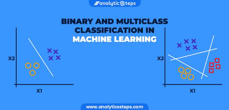
In machine learning, classification is classifying data using certain input variables. A dataset with labels given (training dataset) is used to train the model in a way that the model can provide labels for datasets that are not yet labeled.
Under classification, there are 2 types of classifiers:
- Binary Classification
- Multi-Class Classification
Here let’s discuss Binary classification in detail.
Binary classification is classifying the elements into 2 groups (also called classes or categories) using classification algorithms. Examples of binary classification are:
Algorithms that support binary classification are
- Logistic Regression
- K-Nearest Neighbors
- Decision Trees
- Support Vector Machines
- Naive Bayes
Certain algorithms are not specific for Binary Classification and can also be used for multi-class classification. For example, Support Vector Machine (SVM).
The statistics version of Binary classification is the Binomial Probability distribution.
Bernoulli Probability Distribution:
Random Variable: Numerical description of the outcome of a particular statistics experiment.
For example:
The outcome can be either heads or tails for a simple Coin toss.
We can define a random variable X
X(Heads) = 1
X(Tails) = 0
This can also be X(Tails)=0 and X(Heads)= 1
Here X can be either 1 or 0.
Bernoulli Trail:
This situation can have only 2 outcomes i.e. Success or Failure.
Success refers to winning, so in the case of Bernoulli trials, it is referred to as the required condition.
For example,
A student passes the exam or fails it.
For a random variable X.
X(Pass)= 1
X(Fails)= 0
So, for the student, X=1 is the desired condition.
Bernoulli Distribution:
When a Bernoulli trial occurs, it is called Bernoulli distribution. It is also a special condition of Binomial Distribution (Where there is only a single trial).
Binomial Distribution:
When more than one Bernoulli Trial occurs, it is called Binomial distribution.
For a random variable X:
X~ Binomial(n,p) such that n is a positive integer and 0 ≼ p ≼ 1
Here n is the number of Bernoulli trials, and p is the probability of success for each trial.
In Mathematical terms, the formula for the probability of X being a success is:
When plotted on a graph, it looks something like this:

Traditionally the binary classification follows this rule and finds the probability of success for each outcome and, based on probability, classifies into Category 1 (Success) or Category 2 (Failure).
Evaluation Metrics for Binary Classification:
Accuracy:
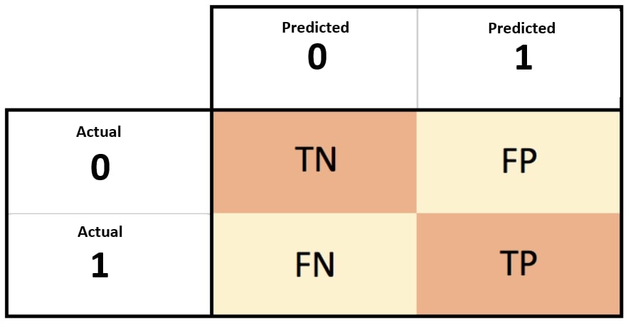
The predicted values can be divided into True Positives, True Negatives, False Positives, and False Negatives.
True Positives (TP): When the model states that the experiment for a particular case is a success and it really is a success.
True Negatives (TN): When the model states that the experiment for a particular case is a failure, it really is a failure.
False Positives (FP): When the model states that the experiment for a particular case is a success, but it is a failure.
False Negatives (FN): When the model states that the experiment for a particular case is a failure, it is a success.
Just to note, the success and failure are references to Bernoulli trials and not the actual success of getting a specific category. It just means the output will be Category 1 or “Not” Category 1 (which is Category 2).
After getting these values, accuracy is:
A confusion matrix is created to analyze these parameters.
Understanding properly with an example and sample code:
Loan Status Prediction:
To check and run the code: https://www.kaggle.com/code/tanavbajaj/loan-status-prediction
As usual, let’s start with importing the libraries and then reading the dataset:
| loan_dataset= pd.read_csv(‘../input/loan-predication/train_u6lujuX_CVtuZ9i (1).csv’) |
This dataset requires some preprocessing because it contains words instead of numbers and some null values.
| # dropping the missing values loan_dataset = loan_dataset.dropna() # numbering the labels loan_dataset.replace({“Loan_Status”:{‘N’:0,’Y’:1}},inplace=True) # replacing the value of 3+ to 4 loan_dataset = loan_dataset.replace(to_replace=’3+’, value=4) # convert categorical columns to numerical values loan_dataset.replace({‘Married’:{‘No’:0,’Yes’:1},’Gender’:{‘Male’:1,’Female’:0},’Self_Employed’:{‘No’:0,’Yes’:1}, ‘Property_Area’:{‘Rural’:0,’Semiurban’:1,’Urban’:2},’Education’:{‘Graduate’:1,’Not Graduate’:0}},inplace=True) |
Here in the first line, NULL values were dropped then the Y and N (representing Yes and No ) in the dataset are replaced by 0 and 1, similarly, other categorical values are also given numbers.
| # separating the data and label X = loan_dataset.drop(columns=[‘Loan_ID’,’Loan_Status’],axis=1) Y = loan_dataset[‘Loan_Status’] X_train, X_test,Y_train,Y_test = train_test_split(X,Y,test_size=0.25,random_state=2) |
As seen in the code the dataset is split into training and testing datasets.
The test_size=0.25 shows that 75% of the dataset will be used for training while 25% for testing.
| model = LogisticRegression() model.fit(X_train, Y_train) |
Sklearn makes it very easy to train the model. Only 1 line of code is required to do so.
Evaluating the model:
| X_train_prediction = model.predict(X_train) training_data_accuracy = accuracy_score(X_train_prediction, Y_train) |
This shows that the accuracy of the training data is 82%
| X_test_prediction = model.predict(X_test) test_data_accuracy = accuracy_score(X_test_prediction, Y_test) |
This shows that the accuracy of the training data is 78.3%
| input_data= (1,1,0,1,0,3033,1459.0,94.0,360.0,1.0,2)
# changing the input_data to a numpy array # reshape the np array as we are predicting for one instance prediction = model.predict(input_data_reshaped) |
Here when random input data is given to the trained model, it gives us the output of whether the loan is approved.
Binary classification is a fundamental task in machine learning, where the goal is to classify instances into one of two classes. In this article, we will explore various aspects of binary classification, including evaluation metrics, threshold selection, handling imbalanced data, ROC curve analysis, feature selection, and real-world case studies.
I. Evaluation Metrics for Binary Classification
Evaluation metrics play a crucial role in assessing the performance of a binary classification model. Common metrics include accuracy, precision, recall, F1-score, and the confusion matrix. These metrics provide insights into the model’s ability to correctly classify instances and quantify the trade-offs between different types of errors.
II. Threshold Selection in Binary Classification
In binary classification, predictions are based on a probability threshold. By adjusting this threshold, we can control the trade-off between precision and recall. Techniques such as the receiver operating characteristic (ROC) curve and precision-recall curve help in selecting an optimal threshold for the desired classification performance.
III. Handling Imbalanced Data in Binary Classification
Imbalanced data, where one class is significantly more prevalent than the other, can impact the performance of binary classification models. Techniques such as over-sampling, under-sampling, and the use of specialized algorithms (e.g., SMOTE) can help address class imbalance and improve model accuracy.
IV. Receiver Operating Characteristic (ROC) Curve Analysis
The ROC curve is a graphical representation of the true positive rate (sensitivity) against the false positive rate (1-specificity) at various classification thresholds. It provides a comprehensive analysis of the model’s performance across different thresholds and allows us to choose the threshold that optimizes the desired trade-off.
V. Feature Selection and Importance in Binary Classification
Feature selection is the process of identifying the most relevant features that contribute to the binary classification task. Techniques such as univariate selection, recursive feature elimination, and feature importance based on tree-based models can help identify the most informative features and improve model performance.
VI. Case Studies: Applications of Binary Classification
Real-world case studies demonstrate the practical applications of binary classification. Examples include spam detection, credit risk assessment, fraud detection, disease diagnosis, sentiment analysis, and churn prediction. These case studies provide insights into the challenges and techniques specific to different domains.
In conclusion, binary classification is a fundamental task in machine learning with diverse evaluation metrics, threshold selection techniques, handling imbalanced data strategies, ROC curve analysis, and feature selection methods. Understanding these aspects and their applications through case studies is essential for building accurate and robust binary classification models in various domains.
FAQs
What is Binary Classification?
Binary Classification is a machine learning task where the goal is to classify instances into one of two classes or categories.
How does Binary Classification differ from multi-class classification?
Binary classification involves distinguishing between two classes, while multi-class classification involves distinguishing between three or more classes.
What are some common algorithms used for Binary Classification?
Common algorithms include Logistic Regression, Decision Trees, Random Forest, Support Vector Machines (SVM), k-Nearest Neighbors (kNN), and Neural Networks (e.g., Perceptron).
How do algorithms handle Binary Classification tasks?
Algorithms are trained to learn a decision boundary that separates the two classes based on input features, using optimization techniques to minimize a chosen loss function.
What evaluation metrics are used for Binary Classification?
Evaluation metrics include accuracy, precision, recall, F1-score, ROC curve, and AUC (Area Under the ROC Curve) for assessing model performance in distinguishing between positive and negative classes.
Can feature engineering techniques be applied to Binary Classification?
Yes, feature engineering techniques such as normalization, feature scaling, dimensionality reduction, and feature selection are applicable to binary classification to improve model performance.
What are some real-world applications of Binary Classification?
Binary classification finds applications in various domains such as spam detection, fraud detection, disease diagnosis, sentiment analysis, and customer churn prediction.