
Lets us try to implement logistic regression from scratch in python.
Recommended to be read after the Neural Networks release.
Importing necessary libraries
The dataset we will be using is Pima-Indians-diabetes-database
Whose objective is to predict whether or not a patient has diabetes diagnostically.
| y = data.Outcome.values x_data = data.drop([“Outcome”],axis=1) |
After this, the data is divided into y, which is the desired classification value column, and x_data, which refers to the various feature of the dataset.
Normalization of the data
The value of column DiabetesPedigreeFunction varies from 0.08 to 2.48, while Insulin varies from 0 to 848. We normalize data to give equal weightage to both the columns
| x = (x_data – np.min(x_data)) / (np.max(x_data) – np.min(x_data)).values |
Upon normalization, the data is converted to the range of 0 – 1.
After this, data is split into training and testing datasets
| from sklearn.model_selection import train_test_split
x_train, x_test, y_train, y_test = train_test_split(x,y,test_size = 0.25, random_state = 42) x_train = x_train.T |
We do this using the built-in method inside the sklearn library.
Defining Necessary Functions

Initialize the weights and biases
The weights and biases are called the parameter of the model. Each feature in the training dataset is given a certain weight. Let’s start by assigning them some random value, i.e., 0.01.
| def initialize_weights_and_bias(dimension):
w = np.full((dimension,1),0.01) |
Sigmoid function
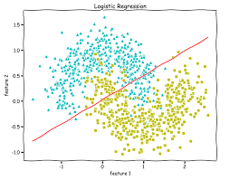
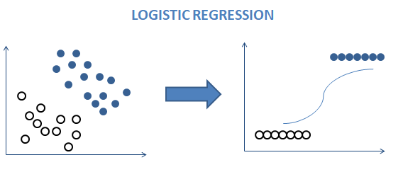
Logistic regression uses regression to predict the label by making a linear decision boundary. It would make no sense to get a value greater than 1 or less than 0. Here the sigmoid function comes into play. This function ranges between 0 to 1 and is stated as
| def sigmoid(z):
y_head = 1 / (1+np.exp(-z)) return y_head |
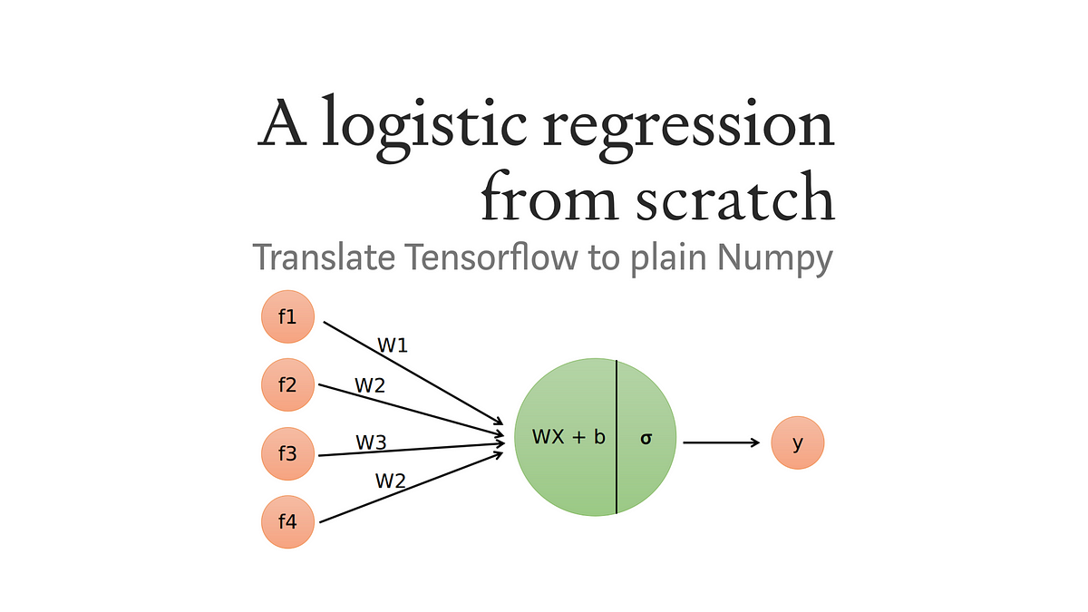
To get the value of the parameter z used in the sigmoid function, we use the formula where x is the features array, w weights, and b is the bias. Now to make our model learn, we need to punish it for the losses and penalize it for wrong predictions this is done by the loss function, which is stated as
And cost function is effectively the sum of loss across all the cases.
This process of penalizing the model and moving forward with the predictions is known as forward propagation.
If we recall, we allotted random weights to the parameter; they now will be updated based on our loss function and cost function. To minimize loss and cost function, we use gradient descent which is where w denotes the weights, denotes the stepsize or the factor by which to change the gradient to find the local minima, which are multiplied by the derivative of the loss function to sum it all up, the algorithm works as follows:-
We assume a random datapoint in our graph and calculate its slope; then, we find the direction in which the loss function decreases and update the weights using the gradient descent formula this process is known as backpropagation; we then select a point by taking a stepsize of and repeat this entire process once again sometimes is also referred to as learning rate.
Finally, we write the code for forward and backward propagation combined, as backward propagation also uses the same z found in forward propagation.
| def forward_backward_propagation(w,b,x_train,y_head):
z = np.dot(w.T,x_train) + b #backward propogation |
After we have calculated our parameters, we need to update the randomly assigned weights to do this; we use another update function
| def update(w, b, x_train, y_train, learning_rate,number_of_iterarion): cost_list = [] cost_list2 = [] index = [] # updating(learning) parameters is number_of_iterarion times for i in range(number_of_iterarion): # make forward and backward propagation and find cost and gradients cost,gradients = forward_backward_propagation(w,b,x_train,y_train) cost_list.append(cost) # lets update w = w – learning_rate * gradients[“derivative_weight”] b = b – learning_rate * gradients[“derivative_bias”] if i % 10 == 0: cost_list2.append(cost) index.append(i) print (“Cost after iteration %i: %f” %(i, cost)) parameters = {“weight”: w,”bias”: b}return parameters, gradients, cost_list |
After this function is called, our model has successfully calculated the weights and biases values using forward and backward propagation methods. This process is also used in neural networks i.e. they repeatedly update weights using forward and backward propagation.
Now onto the most awaited part of generating the predictions; we do that by defining a predict function as follows
| def predict(w,b,x_test): # x_test is a input for forward propagation z = sigmoid(np.dot(w.T,x_test)+b) Y_prediction = np.zeros((1,x_test.shape[1])) # if z is bigger than 0.5, our prediction is one means has diabete (y_head=1), # if z is smaller than 0.5, our prediction is zero means does not have diabete (y_head=0), for i in range(z.shape[1]): if z[0,i]<= 0.5: Y_prediction[0,i] = 0 else: Y_prediction[0,i] = 1return Y_prediction |
Combining all the functions
| def logistic_regression(x_train, y_train, x_test, y_test, learning_rate , num_iterations): # initialize dimension = x_train.shape[0] w,b = initialize_weights_and_bias(dimension)parameters, gradients, cost_list = update(w, b, x_train, y_train, learning_rate,num_iterations)y_prediction_test = predict(parameters[“weight”],parameters[“bias”],x_test)# Print train/test Errors print(“————————————-“) print(“test accuracy: {} %”.format(100 – np.mean(np.abs(y_prediction_test – y_test)) * 100)) |
| from sklearn.linear_model import LogisticRegression lr = LogisticRegression() lr.fit(x_train.T,y_train.T) print(“Test Accuracy {}”.format(lr.score(x_test.T,y_test.T))) |
That was all about Logistic Regression without inbuilt python libraries (sklearn).
Building the Logistic Regression Algorithm from Scratch
Logistic Regression is a popular machine learning algorithm used for binary classification problems. In this section, we will delve into building the Logistic Regression algorithm from scratch. By understanding the underlying principles and implementing it ourselves, we gain a deeper insight into its mechanics.
Logistic Function (Sigmoid):
The logistic function, also known as the sigmoid function, is a crucial component of Logistic Regression. It maps any real-valued number to a value between 0 and 1, making it suitable for classification.
You can define the sigmoid function as:
sigmoid(z) = 1 / (1 + e^(-z))
where z is the linear combination of input features and their respective weights.
Hypothesis:
The hypothesis in Logistic Regression is defined as:
h(x) = sigmoid(X * θ)
where X represents the input feature matrix, and θ represents the vector of weights.
Cost Function:
The cost function measures the performance of the model and is crucial for training. In Logistic Regression, you can define the cost function as the average of the negative log-likelihood of the predicted probabilities.
J(θ) = (-1/m) * Σ [y * log(h(x)) + (1-y) * log(1 - h(x))]
where m is the number of training examples, y is the actual label (0 or 1), and h(x) is the predicted probability.
Gradient Descent:
To minimize the cost function and find the optimal weights, we use the gradient descent algorithm. The gradient of the cost function with respect to the weights is computed as:
∇J(θ) = (1/m) * X^T * (h(x) - y)
where X is the input feature matrix, (h(x) – y) represents the error, and X^T is the transpose of X.
Data Preprocessing for Logistic Regression
Data preprocessing is an important step to ensure the accuracy and efficiency of the Logistic Regression model. Here are some key preprocessing steps:
- Data Cleaning: Handle missing values, outliers, and irrelevant data. Remove or impute missing values, and detect and address outliers appropriately.
- Feature Scaling: Normalize or standardize the input features to ensure they have a similar scale. This prevents features with larger values from dominating the training process.
- Feature Engineering: Create new features or transform existing ones to improve the model’s performance. This could involve polynomial features, interaction terms, or other domain-specific transformations.
Cost Function and Gradient Descent in Logistic Regression
The cost function and gradient descent algorithm are essential components of Logistic Regression. The cost function quantifies the error between the predicted probabilities and the actual labels, while gradient descent updates the weights iteratively to minimize the cost function.
Implementing the Training Algorithm
To implement the training algorithm, follow these steps:
- Initialize the weights (θ) with random values.
- Calculate the hypothesis using the sigmoid function.
- Compute the cost function based on the predicted probabilities and actual labels.
- Update the weights using gradient descent by subtracting the gradient multiplied by the learning rate.
- Repeat steps 2 to 4 until convergence or a predefined number of iterations.
Evaluating the Logistic Regression Model
After training the model, it’s crucial to evaluate its performance. Common evaluation metrics for Logistic Regression include accuracy, precision, recall, and F1-score. Additionally, use techniques like cross-validation or holdout validation to assess the model’s generalization ability.
Case Study: Applying Logistic Regression to a Real-World Dataset
To solidify our understanding, let’s apply Logistic Regression to a real-world dataset. Consider a dataset of customer churn in a telecommunications company. We can use Logistic Regression to predict whether a customer will churn or not based on features like contract type, monthly charges, and customer demographics.
- Perform data preprocessing, including handling missing values, scaling features, and encoding categorical variables.
- Implement the Logistic Regression algorithm from scratch using the steps outlined earlier.
- Split the dataset into training and testing sets.
- Train the model using the training set and evaluate its performance on the testing set using appropriate evaluation metrics.
- Analyze the results, interpret the weights, and draw insights about the factors influencing customer churn.
In conclusion, building Logistic Regression from scratch provides a comprehensive understanding of its inner workings. By implementing the algorithm step by step and applying it to a real-world dataset, we gain practical experience in developing and evaluating a Logistic Regression model. This knowledge serves as a foundation for further exploration into more advanced machine-learning techniques.
FAQs
What is Logistic Regression?
Logistic Regression is a statistical method used for binary classification tasks, where the outcome variable takes on only two possible values, typically represented as 0 and 1.
How does Logistic Regression differ from Linear Regression?
While Linear Regression predicts continuous values, Logistic Regression predicts the probability of an observation belonging to a certain class, using the logistic function to constrain predictions between 0 and 1.
How does Logistic Regression work?
Logistic Regression uses the logistic function (also known as the sigmoid function) to map the input features to a probability score, which is then converted into a class label using a threshold value.
How are the parameters (weights and bias) of Logistic Regression learned?
The parameters of Logistic Regression are learned through an optimization process called gradient descent, where the objective is to minimize a cost function such as the binary cross-entropy loss.
Can Logistic Regression handle multi-class classification tasks?
Yes, Logistic Regression can be extended to handle multi-class classification tasks using techniques like one-vs-rest or softmax regression.
What are some common applications of Logistic Regression?
Logistic Regression is widely used in various fields, including healthcare (e.g., disease diagnosis), finance (e.g., credit risk assessment), marketing (e.g., customer churn prediction), and natural language processing (e.g., sentiment analysis).