
In supervised learning, overfitting is a major problem. When it comes to regression trees, it becomes more obvious to prevent this, we specify the Seth of the tree, but there is still a high chance of the dataset being overfitted. To avoid this, we use a random first regressor.
Before understanding how and why this algorithm prevents overfitting, we need to understand certain terms.
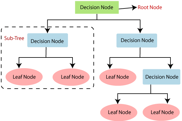
- Decision tree – form the base of the algorithm. As the name suggests decision tree creates a tree-like structure that asks a bunch of questions and tries to predict the result. In other words, it can be understood as a bucket load of nested if-else statements.
If we think the decision tree is highly sensitive to the input dataset, that is, it has high variance let’s understand using an example.
Notebook to test and run code: https://www.kaggle.com/code/tanavbajaj/random-forest/notebook
If we consider a random dataset like
| id | x1 | x2 | x3 | x4 | y |
| 1 | 2.33 | 4.3 | 3.31 | 8.99 | 5.4 |
| 2 | 2.5 | 5.9 | 6.47 | 10.16 | 7.8 |
| 3 | 1.61 | 9.9 | 3.02 | 11.29 | 1.2 |
| 4 | 8.39 | 7.6 | 2.15 | 7.56 | 4.4 |
| 5 | 4.26 | 9.9 | 4.79 | 5.97 | 10.2 |
| 6 | 3.35 | 1.9 | 8.79 | 7.88 | 10.6 |
| 7 | 5.29 | 2.8 | 7.05 | 8.05 | 4.9 |
| 8 | 9.74 | 4.0 | 1.17 | 4.14 | 8.7 |
| 9 | 6.6 | 2.8 | 4.17 | 11.0 | 11.0 |
| 10 | 2.08 | 6.4 | 3.18 | 11.01 | 3.6 |
| 11 | 8.36 | 2.6 | 4.76 | 12.94 | 11.9 |
| 12 | 9.74 | 1.5 | 7.44 | 14.82 | 8.9 |
| 13 | 1.02 | 6.1 | 8.83 | 13.84 | 1.5 |
| 14 | 9.05 | 6.6 | 5.36 | 8.64 | 1.4 |
| 15 | 7.89 | 2.2 | 5.31 | 5.26 | 7.3 |
| 16 | 6.44 | 2.9 | 4.02 | 14.46 | 8.1 |
| 17 | 5.94 | 9.4 | 5.05 | 2.94 | 8.5 |
| 18 | 4.12 | 9.1 | 9.4 | 2.23 | 6.7 |
| 19 | 7.71 | 1.1 | 5.98 | 7.29 | 1.8 |
| 20 | 4.97 | 1.4 | 6.49 | 12.96 | 11.1 |
And try to run the decision tree over it and generate the decision tree it might be something like
| x = data.iloc[:,1:5] y = data.iloc[:,-1] from sklearn.model_selection import train_test_split X_train, X_test, y_train, y_test = train_test_split( x, y, test_size=0.5,random_state=55)From sklearn.tree import DecisionTreeRegressorregressor = DecisionTreeRegressor(random_state=4,max_depth=2) regressor.fit(X_train, y_train)from sklearn.tree import export_graphviz export_graphviz(regressor, out_file =’tree1.dot’) |
Now, if I swap the data x1 and x2 in rows 6, 7 ,8,9
| tmp = x.iloc[5:9,0].copy(deep=True)
x.iloc[5:9,0] = x.iloc[5:9,1] x.iloc[5:9,1] = tmp |
Upon retraining the model and generating the tree
| X_train, X_test, y_train, y_test = train_test_split( x, y, test_size=0.5,random_state=55)
regressor_second = DecisionTreeRegressor(random_state=4,max_depth=2) regressor_second.fit(X_train, y_train) export_graphviz(regressor_second, out_file =’tree2.dot’) with open(“tree2.dot”) as f: dot_graph = f.read() graphviz.Source(dot_graph).view() |
The tree changes to
This shows us that the decision tree is highly sensitive to the dataset.
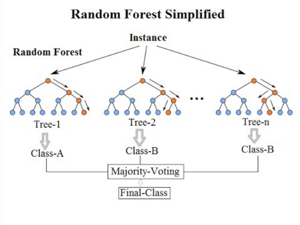
If we dive into a random forest, intuitively, it suggests that it might be some collection of trees, and this presumption is partially correct. A collection makes random forests of various decision trees. Now we may ask if we create trees using the same dataset, wouldn’t they all end up being the same and result in the same variance in the output? Here comes another term from the name into play that is Random. The algorithm uses a method of Bootstrapping. In bootstrapping, the algorithm randomly selects the subsets of the dataset over the number of iterations it is specified to.
To strengthen it more, it then uses another technique called Aggregation. In this, it randomly selects the number of specified features and generates the trees; what this does is it creates a large number of decision trees.
Some trees use the feature with more dominance, thus overfitting the dataset. In contrast, some trees use the worst combination of the feature and give the worst prediction in the result of all the trees being averaged out and predicted as the answer. This algorithm works on the principle of crowd wisdom.
Together the process of Bootstrapping and Aggregating is called Bagging.
As a result, in our random forest, we ended up with trees that employ distinct features for decision-making and were trained on various datasets (due to bagging).
Limitation of random forest
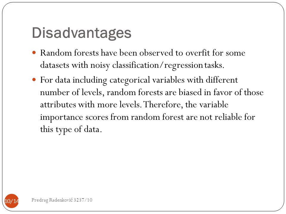
Extrapolation-
When we use the random forest, we often end up extrapolating the values far from the training dataset that is, if the dataset is not present in the training dataset, it will classify it all as the same.
Random forest’s key restriction is that many trees might render the process too sluggish and useless for real-time forecasts. These algorithms are generally quick to train but slow to generate predictions once trained. A more precise prediction needs more trees, resulting in a slower model. The random forest technique is fast enough for most real-world applications, but there may be cases when run-time speed is essential, and other approaches would be preferable.
Feature Importance: Examining the Importance of Features in Random Forest
Examining the Importance of Features in Random Forest
Random Forest provides a useful measure of feature importance, which helps identify the most relevant features for making predictions. The feature importance in Random Forest is derived from the collective contribution of individual decision trees within the ensemble. By aggregating the information from multiple trees, Random Forest can provide a robust estimate of feature importance.
One common metric used to assess feature importance in Random Forest is the mean decrease impurity or Gini importance. It measures the extent to which a feature decreases the impurity or randomness in the predictions. Features that consistently contribute to reducing impurity across multiple trees are considered more important.
Random Forest also enables the calculation of feature importance based on the mean decrease in accuracy or mean decrease in node impurities. These metrics provide insights into the impact of each feature on the overall performance of the model.
By analyzing feature importance in Random Forest, data scientists and analysts can prioritize features for further investigation, feature selection, or focus their efforts on the most influential variables. This understanding aids in better understanding the underlying relationships within the data and improving the interpretability of the model.
Handling Missing Data and Outliers: Addressing the Robustness of Random Forest to Missing Data and Outliers
Random Forest is known for its robustness to missing data and outliers, making it a popular choice in practical applications. Random Forest can handle missing data by utilizing the proximity-based imputation approach. During training, if a sample has missing values for a particular feature, the algorithm will estimate the missing value by considering the values of other features in that sample. This approach helps preserve the integrity of the dataset and ensures that valuable information is not discarded due to missing values.
In terms of outliers, Random Forest is less susceptible to their influence compared to some other algorithms, such as linear regression. The reason lies in the nature of the ensemble learning methodology. Outliers are likely to affect individual decision trees, but their impact is diminished when predictions are averaged across multiple trees. This averaging process helps reduce the influence of outliers and produces more robust predictions.
However, it is still important to preprocess the data and handle outliers appropriately before applying Random Forest. Outliers can distort the relationships between features and the target variable, affecting the overall performance of the model. Therefore, outlier detection techniques or other preprocessing methods can be applied to ensure the best possible results.
Hyperparameter Tuning: Optimizing the Performance of Random Forest through Hyperparameter Tuning
Hyperparameter tuning plays a crucial role in optimizing the performance of Random Forest. Hyperparameters are settings or configurations that are not learned from the data but are defined by the user. They significantly impact the behavior and performance of the Random Forest model.
Some important hyperparameters in Random Forest include the number of trees (n_estimators), the maximum depth of each tree (max_depth), the minimum number of samples required to split an internal node (min_samples_split), and the number of features to consider when looking for the best split (max_features), among others.
Hyperparameter tuning involves searching for the best combination of hyperparameter values to improve the model’s performance. This process can be done using techniques such as grid search, random search, or Bayesian optimization. By systematically exploring different hyperparameter configurations and evaluating their impact on model performance, the optimal set of hyperparameters can be identified.
Tuning the hyperparameters helps prevent overfitting, improve generalization, and enhance the model’s predictive accuracy. It allows the Random Forest to find the right balance between complexity and simplicity, resulting in a more robust and accurate model for a given dataset.
Hyperparameter tuning is an iterative process that requires careful experimentation and evaluation. By selecting the appropriate hyperparameters, practitioners can ensure that the Random Forest model performs optimally and provides the best possible results for their specific use case.
Overfitting and Generalization: Analyzing the Tradeoff between Overfitting and Generalization in Random Forest
Analyzing the Tradeoff between Overfitting and Generalization in Random Forest
Overfitting is a common concern in machine learning models, including Random Forest. Overfitting occurs when the model learns the training data too well, capturing noise or idiosyncrasies that are specific to the training set but do not generalize well to unseen data. Random Forest, with its ensemble approach, offers a natural defense against overfitting.
The random selection of features and bootstrap sampling in Random Forest introduces variability among the individual decision trees. This variability helps to reduce overfitting by averaging out the biases and capturing the general trends in the data. The ensemble nature of Random Forest allows it to strike a balance between complexity and simplicity, thus enhancing generalization.
Random Forest provides built-in mechanisms to control overfitting. By limiting the maximum depth of trees, imposing minimum sample requirements for splitting, or restricting the number of features considered at each split, overfitting can be mitigated. These hyperparameters can be tuned to find the optimal balance between model complexity and generalization.
Interpretability and Model Complexity: Considering the Interpretability and Complexity of Random Forest Models
Considering the Interpretability and Complexity of Random Forest Models
The interpretability of Random Forest models can be more challenging compared to simpler models like linear regression due to their inherent complexity. Random Forest combines multiple decision trees, each making predictions based on different subsets of features and data samples. While this complexity allows Random Forest to capture intricate relationships, it also makes the model less interpretable at an individual tree level.
However, Random Forest still provides interpretability through feature importance measures, which quantify the relative contribution of each feature to the model’s predictions. These measures help identify influential features and gain insights into the underlying relationships within the data.
In Random Forest, factors such as the number of trees, the depth of each tree, and the number of features considered at each split influence model complexity. Increasing the number of trees or their depth can result in more complex models with a higher capacity to capture intricate patterns in the data. However, overly complex models may be prone to overfitting and can be harder to interpret.
Finding the right balance between model complexity and interpretability depends on the specific use case. In applications where understanding the model is crucial, techniques like partial dependence plots or permutation importance can be used to gain insight into how different features influence predictions.
Practical Applications: Exploring Real-World Use Cases and Applications of Random Forest
Exploring Real-World Use Cases and Applications of Random Forest
Random Forest has gained popularity and has been successfully applied to various real-world problems across domains. Some common applications of Random Forest include:
Predictive Analytics: You can use random Forest in predictive modeling tasks such as predicting customer behavior, credit risk assessment, fraud detection, and demand forecasting. Its ability to handle a large number of features and complex relationships makes it suitable for these applications.
Image and Text Classification: You can employ the random Forest for image and text classification tasks, such as object recognition or sentiment analysis. It can handle high-dimensional data and capture non-linear relationships between features and labels.
Bioinformatics: Random Forest finds applications in genomics, proteomics, and other areas of bioinformatics. It can aid in gene expression analysis, identifying disease biomarkers, and predicting protein structures.
Remote Sensing and Geospatial Analysis: You can utilize random Forest in remote sensing and geospatial analysis tasks, including land cover classification, land use mapping, and environmental monitoring. Its ability to handle multi-dimensional data and capture complex relationships makes it suitable for analyzing satellite imagery and geospatial datasets.
Recommender Systems: you can employ the Random Forest in recommender systems to suggest personalized recommendations to users. By analyzing user behavior and item features, it can predict user preferences and improve the accuracy of recommendations.
Conclusion
Random Forest is a powerful and versatile Machine Learning algorithm used for both classification and regression tasks. It offers great flexibility, scalability as well as accuracy, which makes it an ideal method of choice in many application domains. With the use of random forest we can benefit from various ensemble techniques which increase overall predictive performance. Random Forest also incorporates several important parameters that allow us to reduce overfitting by pruning the trees or adjusting other hyper-parameters such as minimum leaf size, etc. By using these parameters effectively, one can achieve great results in any given task like classification or regression problem.
FAQs
What is Random Forest?
Random Forest is a machine learning algorithm for classification and regression tasks.
How does Random Forest work?
It constructs multiple decision trees during training and outputs the mode of the classes for classification or mean prediction for regression.
When should I use Random Forest?
Use Random Forest when you need robust and accurate predictions from high-dimensional datasets.
How does Random Forest handle overfitting?
It mitigates overfitting by averaging predictions from multiple trees.
Can Random Forest handle missing data?
Yes, Random Forest can handle missing data without imputation.
How do I interpret the results from a Random Forest model?
Feature importance can be determined by assessing the impact of each feature on prediction accuracy.
Is Random Forest suitable for large datasets?
Yes, Random Forest is scalable and can handle large datasets efficiently.